
A Dual Input-aware Factorization Machine for CTR Prediction
Proceedings of the Twenty-Ninth International Joint Conference on Artificial Intelligence. Main track. Pages 3139-3145.
https://doi.org/10.24963/ijcai.2020/434
Keywords
- Multidisciplinary Topics and Applications: Recommender Systems
- Machine Learning: Recommender Systems
- Data Mining: Classification, Semi-Supervised Learning
Abstract
Factorization Machines (FMs) refer to a class of general predictors working with real valued feature vectors, which are well-known for their ability to estimate model parameters under significant sparsity and have found successful applications in many areas such as the click-through rate (CTR) prediction. However, standard FMs only produce a single fixed representation for each feature across different input instances, which may limit the CTR model’s expressive and predictive power. Inspired by the success of Input-aware Factorization Machines (IFMs), which aim to learn more flexible and informative representations of a given feature according to different input instances, we propose a novel model named Dual Input-aware Factorization Machines (DIFMs) that can adaptively reweight the original feature representations at the bit-wise and vector-wise levels simultaneously. Furthermore, DIFMs strategically integrate various components including Multi-Head Self-Attention, Residual Networks and DNNs into a unified end-to-end model. Comprehensive experiments on two real-world CTR prediction datasets show that the DIFM model can outperform several state-of-the-art models consistently.
- [Amodei et al., 2016] Dario Amodei, Sundaram Anantha- narayanan, Rishita Anubhai, Jingliang Bai, Eric Batten- berg, Carl Case, Jared Casper, Bryan Catanzaro, Qiang Cheng, Guoliang Chen, et al. Deep speech 2: End-to- end speech recognition in english and mandarin. In Inter- national conference on machine learning, pages 173-182, 2016.
- [Cheng et al., 2016] Heng-Tze Cheng, Levent Koc, Jeremiah Harmsen, Tal Shaked, Tushar Chandra, Hrishi Aradhye, Glen Anderson, Greg Corrado, Wei Chai, Mustafa Ispir, et al. Wide & deep learning for recom- mender systems. In Proceedings of the 1st workshop on deep learning for recommender systems, pages 7-10. ACM, 2016.
- [Cho et al., 2014] Kyunghyun Cho, Bart Van Merriënboer, Caglar Gulcehre, Dzmitry Bahdanau, Fethi Bougares, Holger Schwenk, and Yoshua Bengio. Learning phrase representations using rnn encoder-decoder for statistical machine translation. arXiv preprint arXiv:1406.1078, 2014.
- [Guo et al., 2017] Huifeng Guo, Ruiming Tang, Yunming Ye, Zhenguo Li, and Xiuqiang He. Deepfm: a factorization-machine based neural network for ctr predic- tion. arXiv preprint arXiv:1703.04247, 2017. IJCAI
- [He and Chua, 2017] Xiangnan He and Tat-Seng Chua. Neu- ral factorization machines for sparse predictive analytics. In Proceedings of the 40th International ACM SIGIR con- ference on Research and Development in Information Re- trieval, pages 355-364. ACM, 2017.
- [He et al., 2016] Kaiming He, Xiangyu Zhang, Shaoqing Ren, and Jian Sun. Deep residual learning for image recog- nition. In Proceedings of the IEEE conference on CVPR, pages 770-778, 2016.
- [Juan et al., 2016] Yuchin Juan, Yong Zhuang, Wei-Sheng Chin, and Chih-Jen Lin. Field-aware factorization ma- chines for ctr prediction. In Proceedings of the 10th ACM Conference on Recommender Systems, pages 43-50. ACM, 2016.
- [Kingma and Ba, 2014] Diederik P Kingma and Jimmy Ba. Adam: A method for stochastic optimization. arXiv preprint arXiv:1412.6980, 2014.
- [Lee et al., 2012] Kuang-chih Lee, Burkay Orten, Ali Das- dan, and Wentong Li. Estimating conversion rate in dis- play advertising from past erformance data. In Proceed- ings of the 18th ACM SIGKDD international conference on Knowledge discovery and data mining, pages 768-776. ACM, 2012.
- [Lian et al., 2018] Jianxun Lian, Xiaohuan Zhou, Fuzheng Zhang, Zhongxia Chen, Xing Xie, and Guangzhong Sun. xdeepfm: Combining explicit and implicit feature inter- actions for recommender systems. In Proceedings of the 24th ACM SIGKDD International Conference on Knowl- edge Discovery & Data Mining, pages 1754-1763. ACM, 2018.
- [McMahan et al., 2013] H Brendan McMahan, Gary Holt, David Sculley, Michael Young, Dietmar Ebner, Julian Grady, Lan Nie, Todd Phillips, Eugene Davydov, Daniel Golovin, et al. Ad click prediction: a view from the trenches. In Proceedings of the 19th ACM SIGKDD in- ternational conference on Knowledge discovery and data mining, pages 1222-1230. ACM, 2013.
- [Qu et al., 2016] Yanru Qu, Han Cai, Kan Ren, Weinan Zhang, Yong Yu, Ying Wen, and Jun Wang. Product- based neural networks for user response prediction. In 2016 IEEE 16th ICDM, pages 1149-1154. IEEE, 2016.
- [Rendle, 2010] Steffen Rendle. Factorization machines. In 2010 IEEE ICDM, pages 995-1000. IEEE, 2010.
- [Song et al., 2019] Weiping Song, Chence Shi, Zhiping Xiao, Zhijian Duan, Yewen Xu, Ming Zhang, and Jian Tang. Autoint: Automatic feature interaction learning via self-attentive neural networks. In Proceedings of the 28th CIKM, pages 1161-1170. ACM, 2019.
- [Vaswani et al., 2017] Ashish Vaswani, Noam Shazeer, Niki Parmar, Jakob Uszkoreit, Llion Jones, Aidan N Gomez, Łukasz Kaiser, and Illia Polosukhin. Attention is all you need. In Advances in neural information processing sys- tems, pages 5998-6008, 2017.
- [Wang et al., 2017] Ruoxi Wang, Bin Fu, Gang Fu, and Min- gliang Wang. Deep & cross network for ad click predic- tions. In Proceedings of the ADKDD'17, page 12. ACM, 2017.
- [Wen et al., 2019] Hong Wen, Jing Zhang, Quan Lin, Keping Yang, and Pipei Huang. Multi-level deep cascade trees for conversion rate prediction in recommendation system. In Proceedings of the AAAI Conference on Artificial Intelli- gence, volume 33, pages 338-345, 2019.
- [Xiao et al., 2017] Jun Xiao, Hao Ye, Xiangnan He, Han- wang Zhang, Fei Wu, and Tat-Seng Chua. Atten- tional factorization machines: Learning the weight of fea- ture interactions via attention networks. arXiv preprint arXiv:1708.04617, 2017. IJCAI
- [Yu et al., 2019] Yantao Yu, Zhen Wang, and Bo Yuan. An input-aware factorization machine for sparse prediction. In Proceedings of the 28th IJCAI, pages 1466-1472. AAAI Press, 2019. IJCAI
- [Zhang et al., 2016] Weinan Zhang, Tianming Du, and Jun Wang. Deep learning over multi-field categorical data. In European conference on information retrieval, pages 45- 57. Springer, 2016.
- [Zhou et al., 2018] Guorui Zhou, Xiaoqiang Zhu, Chenru Song, Ying Fan, Han Zhu, Xiao Ma, Yanghui Yan, Junqi Jin, Han Li, and Kun Gai. Deep interest network for click- through rate prediction. In Proceedings of the 24th ACM SIGKDD International Conference on Knowledge Discov- ery & Data Mining, pages 1059-1068. ACM, 2018.
- [Zhou et al., 2019] Guorui Zhou, Na Mou, Ying Fan, Qi Pi, Weijie Bian, Chang Zhou, Xiaoqiang Zhu, and Kun Gai. Deep interest evolution network for click-through rate pre- diction. In Proceedings of the AAAI Conference on Artifi- cial Intelligence, volume 33, pages 5941-5948, 2019.
References were extracted automatically from the PDF and may contain errors.
Full text extracted automatically from the PDF; figures, tables and equations may differ. The PDF is the version of record.
1 Introduction
The prediction of click-through rate (CTR) is crucial in online advertising [McMahan et al., 2013; Juan et al., 2016; Wen et al., 2019], where the task is to estimate the probability that a user will click on a recommended ad or item. In online advertising, advertisers pay publishers to display their ads on publishers' sites. One popular payment model is the cost-per-click (CPC) model [Zhou et al., 2018; Zhou et al., 2019], where advertisers are charged only when a click occurs. As a consequence, a publisher's revenue relies heavily on the ability to predict CTR accurately [Wang et al., 2017].
Representing features accurately is important for CTR prediction. Typically, each feature is represented as a scalar weight and a k-dimensional embedding vector in Factorization Machines (FMs)-based models [Rendle, 2010], such as AFM [Xiao et al., 2017], NFM [He and Chua, 2017], DeepFM [Guo et al., 2017] and xDeepFM [Lian et al., 2018]. However, in all the above models, the same representation of a given feature is shared among different input instances (a.k.a. different scenes), which may limit the CTR model's predictive power. For example, the feature female is apparently crucial for click probability in the instance: {young, female, student, pink, skirt}. However, in another instance: {young, female, student, blue, notebook}, the feature female is relatively less crucial. As such, the representation of a given feature in different input instances (e.g., the feature female in the above two instances) should be assigned different levels of predictive power. To this end, IFMs were proposed [Yu et al., 2019], which consider the uniqueness of each input instance and learn a unique input-aware factor (used to reweight the original feature representations) for the same feature in different input instances via DNNs.
∗Corresponding Author
Despite great promise, we argue that, in IFMs, plain DNNs implicitly learn the input-aware factors at the bit-wise level. That is to say, all the elements within the same embedding vector will affect each other. Meanwhile, in the field of CTR prediction, whether DNNs are the most effective model in learning the input-aware factors remains an open question. After all, the bit-wise level learning itself may be insufficient for achieving optimal prediction.
Inspired by the success of Transformer in machine translation tasks [Vaswani et al., 2017], which is highly efficient and capable of uncovering syntactic and semantic patterns among words in a sentence, we adopt its core idea, the Multi-Head Self-Attentionmechanism, to exploit the implicit relationship among features in an instance, and to adaptively learn the input-aware factors at the vector-wise level.
In this paper, in light of the uniqueness of each instance, by allowing the same feature to have different levels of predictive power in different instances, we propose a competent model for CTR prediction tasks named Dual Input-aware Factorization Machines (DIFMs). It shares the same benefits as the DNNs model (i.e., the IFM model) and introduces a novel vector-wise network that is more effective in learning the input-aware factors for reweighting the original feature representations. To summarize, we make the following key contributions:
- We propose a novel network model DIFMs, which can adaptively learn different representations of a given feature according to different input instances effectively.
- Compared to the IFMmodel, our proposed DIFMmodel can effectively learn the input-aware factors (used to reweight the original feature representations) at the bitwise and vector-wise levels simultaneously.
- The DIFM model strategically integrates various components including Multi-Head Self-Attention, Residual Networks and DNNs into a unified end-to-end model.
- We conduct comprehensive experiments on two realworld CTR prediction datasets, and the results confirm that our DIFM model can outperform major state-of-theart models consistently.
2 FactorizationMachines
As a class of general predictors working with real valued feature vectors, Factorization Machines (FMs) are able to estimate parameters under significant sparsity effectively. Formally, FMs predict the target as:
where w0 is the global bias, wi and vi ∈ Rk denote the scalar weight and the k-dimensional embedding vector of the i-th feature, respectively. 〈vi, vj〉 is the dot product of two vectors of size k, which models the interaction between the i-th and j-th features.
3 Our Approach
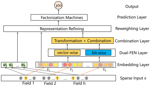
In this section, we present the structure of our proposed DIFM model as shown in Figure 1.
3.1 The DIFMModel
The motivation is to adaptively learn the input-aware factors (used to reweight the original feature representations: w and v) both at the bit-wise and vector-wise levels simultaneously. To this end, we propose the novel Dual Input-aware Factorization Machines (DIFMs) for CTR prediction.
The DIFM model consists of the following components: (1) Sparse Input and Embedding Layer; (2) Dual-Factor Estimating Networks (Dual-FEN) Layer; (3) Combination Layer; (4) Reweighting Layer; (5) Prediction Layer.
Sparse Input and Embedding Layer
The sparse input layer and embedding layer are widely used in deep learning based CTR models such as DeepFM [Guo et al., 2017] and AFM [Xiao et al., 2017]. The sparse input layer adopts a sparse representation for raw input features. The embedding layer is able to embed the sparse feature into a low dimensional, dense real-value vector. The output of the embedding layer is a concatenated field embedding vector: Ex = [vT 1 , vT 2 , · · · , vT i , · · · , vT h ], where h denotes the number of fields while vi ∈ Rk denotes the embedding vector of the i-th field , and k is the embedding size.
Dual-FEN Layer
The Dual-FEN Layer consists of two components 1 : the vector-wise part and the bit-wise part, which both aim to learn a unique input-aware factor for the same feature in different input instances.
The vector-wise part is inspired by the success of Transformer for machine translation in natural language processing (NLP) [Vaswani et al., 2017]. In this work, we adopt its core idea, the Multi-Head Self-Attention mechanism, to learn the input-aware factors at the vector-wise level. Figure 2 shows the structure of the vector-wise part.
First, we need to reshape the embedding vector Ex into a h × k matrix, which is the input of the vector-wise part.
Next, we map the input matrix into three different matrices: Qi (Queries), Ki (Keys), Vi (Values) for the i-th head (a.k.a. the i-th subspace):
where the projection matrices WQi , WKi ∈ Rk×dk , WVi ∈ Rk×dv , and dk denotes the size of the attention factor (in general, dk = dv). Then, according to Scaled Dot-Product Attention [Vaswani et al., 2017], we conduct the dot products of the Query with all Keys divided by √dk, and apply a softmax function to obtain the weights on Values:
As the original paper [Vaswani et al., 2017] suggests, it is beneficial to linearly project the Queries, Keys and Values n times with different, learned linear projections to dk, dk and dv dimensions, respectively. On each of these projected Queries, Keys and Values, we perform the attention function in parallel, yielding a set of dv-dimensional vectors and concatenate them:
1 For simplicity of writing, we use "vec" denotes "vector-wise" and "bit" denotes "bit-wise" in formulas.
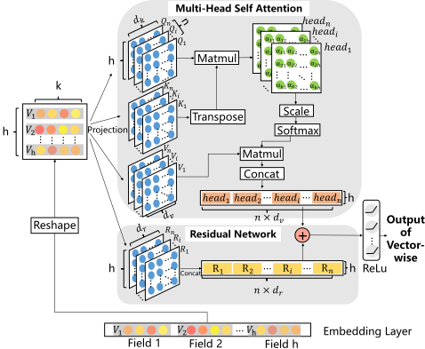
where headi ∈ Rh×dv denotes the output of the i-th single head and n is the number of heads. MultiHead(Uvec) ∈ Rh×(dv×n) denotes the output of Multi-Head Self-Attention.
To preserve some information about the original embedding vector, after the Multi-Head Self-Attention, we use the Residual Network to add the original feature embedding vector to the output of Multi-Head Self-Attention:
where WRi ∈ Rk×dr denotes the linear projection by the shortcut connections to match the dimensions. Ri ∈ Rh×dr is the i-th residual block related to headi. Note that, to keep dimensions consistent, we set dr = dk = dv. Finally, the output of the vector-wise part can be formulated as:
where Ovec ∈ Rh×(dv×n) and σ is the activation function.
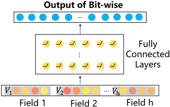
The bit-wise part is a stack of fully connected layers. The input of the bit-wise part: Ibit = Ex. Figure 3 shows the structure of the bit-wise part.
where Ibit ∈ R(h×k) is the input of the bit-wise part, andWi, bi, σi, ai denote the weight matrix, bias vector, activation function and the output of the i-th layer, respectively. The output of the bit-wise part Obit ∈ Rt where t is the number of neurons of the last hidden layer is defined as:
Combination Layer
In this layer, the output of the vector-wise part is reshaped into the form of a single vector (i.e., Ovec ∈ Rh1 , Obit ∈ Rh2 , where h1 = h × dv × n and h2 = t).
Then, the two input-aware factors based on the vector-wise and bit-wise parts are calculated as:
where Pvec ∈ Rh1×h and Pbit ∈ Rh2×h are the weight matrices that transformOvec andObit into a h-dimensional vector, respectively. Finally, we combine the two intermediate input-aware factors:
where mx ∈ Rh is the complete input-aware factor corresponding to the sparse input x, which considers both the vector-wise and bit-wise parts.
Reweighting Layer
The definition of the reweighting layer is as follows:
where mx,i is the i-th element in mx, which denotes the i-th input-aware factor for each non-zero feature in x. wx,i, vx,i are the reweighted representations of features for the specific input x, which are more accurate and informative.
Prediction Layer
With the reweighted input-aware weight wx,i and embedding vector vx,i, the final FM prediction score is obtained as:
3.2 Learning
For binary classification, the learning process aims to minimize the following objective function (log loss):
where yi ∈ {0, 1} is the ground truth of the i-th instance while σ( ˆ yi) ∈ (0, 1) is the predicted CTR (here σ is the sigmoid function) and N is the total number of training instances.
3.3 Relationship with FMand IFM
By removing the vector-wise part and Combination Layer, it is easy to see that our DIFM model will be degraded to the IFMmodel. If we further remove the DNNs (bit-wise part) , and at the same time fix all mx,i to 1, wx,i and vx,i will only depend on the i-th feature, and the shallow DIFM model is downgraded to the traditional FMmodel.
4 RelatedWork
Logistic Regression (LR) only models the linear combination of raw features for CTR prediction. FMs [Rendle, 2010] use factorization techniques to model second-order feature interactions and work well on large sparse data. As a variant of FMs, Field-aware FM (FFM) [Juan et al., 2016] allows each feature to have multiple embedding vectors for feature interactions but suffers from the memory requirement.
With the success of deep learning in computer vision, speech recognition, and natural language processing [He et al., 2016; Amodei et al., 2016; Cho et al., 2014], an increasing number of DNN-based models for CTR prediction have been proposed. How to effectively model feature interactions has become the key challenge for most of these models. FNN [Zhang et al., 2016] is a forward neural network using FM to pre-train the embedding layer. PNN [Qu et al., 2016] introduces a product layer between the embedding layer and DNN layers to explore the high-order feature interactions. NFM [He and Chua, 2017] devises a bilinear interaction layer to obtain the element-wise product of pairwise feature interactions and then stacks multiple non-linear layers over the bilinear interaction layer to capture the high-order feature interactions. Wide&Deep [Cheng et al., 2016] comprises the wide and deep parts, where the wide part models the linear low-order feature interactions, and the deep part models the non-linear high-order feature interactions. However, feature engineering is still needed in the wide part. DeepFM [Guo et al., 2017] uses FM to replace the wide part in Wide&Deep without any feature engineering. DCN [Wang et al., 2017] efficiently captures certain bounded-degree feature interactions explicitly. xDeepFM [Lian et al., 2018] also models the loworder and high-order feature interactions in an explicit way by proposing a novel CIN component.
Meanwhile, the attention mechanism is also introduced for CTR prediction. AFM [Xiao et al., 2017] adopts the attention mechanism to model the importance of all feature interactions. AutoInt [Song et al., 2019] combines the multi-head attention and residual networks for feature interactions.
However, in all the above models, the same representation of a given feature is shared in different instances, which may limit the CTR model's predictive power [Yu et al., 2019]. To overcome this limit, IFM [Yu et al., 2019] learns a unique input-aware factor for the same feature in different instances via DNNs. Inspired by the success of IFM, our proposed Dual Input-aware Factorization Machines (DIFMs) can adaptively learn the input-aware factors (used to reweight the original feature representations) at the bit-wise and vector-wise levels simultaneously and effectively.
5 Experiments
In this section, we conduct extensive experiments to answer the following questions:
- RQ1 How do the key hyper-parameters of DIFM (i.e., the number of heads, the attention size dk, activation function and the number of hidden layers) impact its performance?
- RQ2 Is it necessary to combine the bit-wise and vector-wise levels for learning the input-aware factors? Which is the most important component in DIFM?
- RQ3 How does DIFM perform compared to state-of-the-art methods for CTR prediction?
We will answer these questions after presenting some fundamental experimental settings.
5.1 Experimental Settings
Datasets. We evaluate our proposed DIFM model on the following two datasets. Avazu 2 dataset was published in the contest of Avazu Click-Through Rate Prediction in 2014. It contains click logs with 40 millions of data instances. For each click data, there are 24 fields which indicate elements of a single ad impression. We follow the data processing details of IFM [Yu et al., 2019] and split it randomly into two parts: 80% is for training and 20% is for testing. Criteo 3 dataset contains one month of ad click logs. There are 13 continuous features and 26 categorical ones. We select 7 consecutive days of samples for training, and the next 1 day for evaluation. At last, it contains click logs with 100 millions of data instances.
Evaluation Metrics. We use two evaluation metrics in our experiments: AUC (Area Under ROC) and Logloss (cross entropy). Note that an improvement of 0.001-level in AUC or Logloss is usually regarded as being significant for CTR prediction, because it will bring a large increase in a company's revenue if the company has a large user base, which has also been pointed out in many existing works [Cheng et al., 2016; Guo et al., 2017; Wang et al., 2017; Song et al., 2019].
Baselines. We compare our proposedDIFMmodel with the following eight competitive models, some of which are stateof-the-art models for CTR prediction.
- LR [Lee et al., 2012]: Logistic Regression only models the linear combination of raw features.
- FM [Rendle, 2010]: FM uses factorization techniques to model second-order feature interactions.
- FFM [Juan et al., 2016]: FFM introduces field-aware embedding vectors mechanism, which gain FFM higher capacity and better performance. Considering its high space complexity, we set k = 4 in this paper.
- NFM [He and Chua, 2017]: We implement the NeuralFM and set the number of layers in the hidden layer to 1 with 512 neurons as the original paper.
2 http://www.kaggle.com/c/avazu-ctr-prediction
3 http://labs.criteo.com/downloads/
- AFM [Xiao et al., 2017]: AFM extends FM by using attention mechanism to distinguish the different importance of second-order feature interactions.
- DeepFM [Guo et al., 2017]: The FM part is a factorization machine, and the deep part is a three-layer MLP with layer sizes 256, 256, 256.
- xDeepFM [Lian et al., 2018]: xDeepFM considers the implicit and explicit modeling of high-order feature interactions simultaneously, which are implemented with the DNN and CIN components.
- IFM [Yu et al., 2019]: We implement the method with the same structure of the original paper. The hidden dimension in Factor Estimating Network (FEN) is set to 256, 256, 256 as recommended.
Parameter Settings. We implement all models using Tensorflow 4 . To enable a fair comparison, all models are learned by optimizing the log loss (Equation 14) using the Adam (Learning rate: 0.001) optimizer [Kingma and Ba, 2014]. For all methods, the embedding sizes for Criteo and Avazu are set to 20 and 40, respectively, which is the same as the parameter settings in IFM [Yu et al., 2019]. The batch size is set to 2000 for both datasets. The default setting for the number of neurons per layer is: (1) 256 for DNNs layers in DeepFM, xDeepFM, IFM and DIFM; (2) 200 for CIN layers in xDeepFM. For AFM, the attention factor is also set to 256 as the original paper recommended [Xiao et al., 2017]. To be fair and achieve the best performance for each model, hyper-parameters of each model are tuned by grid-searching carefully. The best settings for each model have been shown in corresponding sections.
5.2 Hyper-parameter Study (RQ1)
First, we study the impact of hyper-parameters on DIFM, including (1) the number of attention heads n; (2) the attention key size dk; (3) activation functions (the vector-wise part); (4) the number of hidden layers in DNNs.
To avoid the analysis being affected by the bit-wise part, we conducted experiments (1), (2), (3) via removing the DNNs (bit-wise) part while varying the settings for the vector-wise part. Subsequently, we conducted experiment (4) via holding the best settings for the vector-wise part while varying the settings for the bit-wise part.
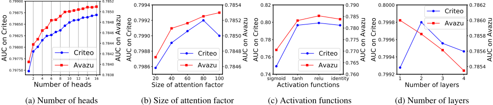
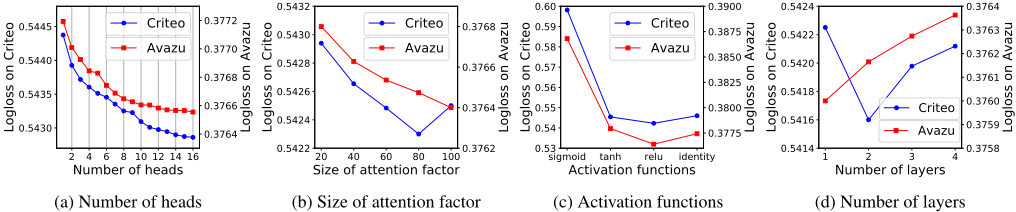
Number of Attention Heads. Figures 4a and 5a demonstrate the impact of the number of self-attention heads. We can observe that model performance on two datasets increases steadily when the number of heads increases from 1 to 16. We also conducted experiments with heads greater than 16, but found that the improvement of further increasing head number is not significant, even the quality will drop off with too many heads. Consequently, we fixed the number of heads to 16 for the following experiments.
Size of Attention Factor. Adding the size of attention factor (dk) equals increasing the number of feature maps in Eq.3. As shown in Figures 4b and 5b, model performance on Avazu dataset increases steadily when we increase the size of attention factor from 20 to 100, while on Criteo dataset, 80 is a more suitable setting for the size of attention factor. As such, To avoid the model being too complicated, we fixed the size of attention factor to 100 for Avazu and 80 for Criteo.
Activation Function. Note that we exploited relu as activation function on neurons of the vector-wise part, as shown in Eq.7. A common practice in deep learning literature is to employ non-linear activation functions on hidden neurons. We thus compared the performance of different activation functions on the vector-wise part (for neurons of the bit-wise part, we keep the activation function with relu). As shown in Figures 4c and 5c, relu is indeed more appropriate for neurons of the vector-wise part.
| Avazu | Criteo | |||
|---|---|---|---|---|
| Model | AUC | Logloss | AUC | Logloss |
| FM | 0.7758 | 0.3822 | 0.7837 | 0.5600 |
| bit-wise | 0.7849 | 0.3771 | 0.7981 | 0.5437 |
| vector-wise-no-res | 0.7851 | 0.3766 | 0.7990 | 0.5425 |
| vector-wise | 0.7853 | 0.3764 | 0.7992 | 0.5423 |
| complete-no-res | 0.7857 | 0.3762 | 0.7996 | 0.5418 |
| complete | 0.7860 | 0.3760 | 0.7998 | 0.5416 |
Depth of Network. Figures 4d and 5d demonstrate the impact of the number of hidden layers in DNNs. For Criteo dataset, the performance of DIFM increases with the depth of network at the beginning. However, the model performance starts to degrade when the depth of network is set to greater than 2. It is caused by overfitting evidenced by the observation that the training error still keeps decreasing. For Avazu dataset, when we stack more layers, the performance is not further improved, and the best performance is when we use only one hidden layer.
5.3 Ablation Study (RQ2)
The DIFM model strategically integrates the bit-wise and vector-wise levels for learning the input-aware factors into a unified end-to-end model. As such, whether it is indeed necessary and effective to combine them for joint prediction? Which is the most important component in our DIFMmodel? To validate and gain deep insights into the DIFM model, we conducted ablation experiments over DIFM. Table 1 shows the performance of DIFM w.r.t. different components (i.e. different variants). We have the following key observations:
- First, introducing the input-aware factors mechanism for reweighting the original feature representations is effective, which can be verified through the fact that all variants of the DIFM model outperform FM by a large margin on both datasets.
- Second, it is necessary and effective to combine the bitwise and vector-wise levels for joint prediction. Considering the bit-wise and vector-wise levels simultaneously for learning the input-aware factors brings additional improvement over the cases of considering either alone.
- Lastly, the vector-wise component is the best individual variant over DIFM, and the residual unit can further improve performance, which demonstrates the importance of preserving some information about the original embedding vector.
| Avazu | Criteo | |||
|---|---|---|---|---|
| Model | AUC | Logloss | AUC | Logloss |
| LR | 0.7505 | 0.3963 | 0.7766 | 0.5670 |
| FM | 0.7758 | 0.3822 | 0.7837 | 0.5600 |
| FFM | 0.7769 | 0.3813 | 0.7976 | 0.5443 |
| AFM | 0.7782 | 0.3805 | 0.7911 | 0.5512 |
| NFM | 0.7816 | 0.3785 | 0.7898 | 0.5528 |
| IFM | 0.7849 | 0.3771 | 0.7981 | 0.5437 |
| DeepFM | 0.7821 | 0.3782 | 0.7975 | 0.5446 |
| xDeepFM | 0.7830 | 0.3778 | 0.7979 | 0.5439 |
| DIFM | 0.7860 | 0.3760 | 0.7998 | 0.5416 |
5.4 Performance Comparison (RQ3)
In this final subsection, we compared our DIFM model with several strong baselines. The performance of different models on Avazu and Criteo datasets is shown in Table 2, from which we have the following key observations:
- First, learning feature interactions improves the performance of CTR prediction models. This observation is from the fact that LR performs far worse than all the rest models. Meanwhile, learning the low-order and highorder feature interactions endows the CTR prediction model better representation ability.
- Second, learning adaptive and different representations of a given feature according to different input instances is crucial in CTR prediction, which can be verified through the result that the shallow DIFM and IFMmodels achieve even better performance than deep learning methods, such as AFM, NFM, DeepFM and xDeepFM.
- Lastly, our proposed DIFMmodel consistently achieves the best performance on both datasets. This demonstrates the effectiveness and rationality of the combination of the bit-wise and vector-wise in the DIFM model.
6 Conclusion
In this paper, we presented a novel model named Dual Inputaware Factorization Machines (DIFMs) for CTR prediction. It aims to adaptively learn flexible representations of a given feature according to different input instances with the help of the Dual-Factor Estimating Network (Dual-FEN). The major advantage of DIFM is that it can effectively learn the inputaware factors (used to reweight the original feature representations) not only at the bit-wise level but also at the vectorwise level simultaneously. Extensive experiments on two real-world CTR prediction datasets were conducted to verify the effectiveness of DIFM for CTR prediction. In terms of two popular evaluation metrics, empirical results indicate that DIFM can outperform the classical LR, FM, FFM and several major state-of-the-art deep learning methods such as AFM, NFM, IFM, DeepFM and xDeepFM consistently.
@inproceedings{ijcai2020p434,
  title     = {A Dual Input-aware Factorization Machine for CTR Prediction},
  author    = {Lu, Wantong and Yu, Yantao and Chang, Yongzhe and Wang, Zhen and Li, Chenhui and Yuan, Bo},
  booktitle = {Proceedings of the Twenty-Ninth International Joint Conference on
               Artificial Intelligence, {IJCAI-20}},
  publisher = {International Joint Conferences on Artificial Intelligence Organization},
  editor    = {Christian Bessiere},
  pages     = {3139--3145},
  year      = {2020},
  month     = {7},
  note      = {Main track},
  doi       = {10.24963/ijcai.2020/434},
  url       = {https://doi.org/10.24963/ijcai.2020/434},
}
TY - CPAPER TI - A Dual Input-aware Factorization Machine for CTR Prediction AU - Lu, Wantong AU - Yu, Yantao AU - Chang, Yongzhe AU - Wang, Zhen AU - Li, Chenhui AU - Yuan, Bo T2 - Proceedings of the Twenty-Ninth International Joint Conference on Artificial Intelligence, IJCAI-20 PB - International Joint Conferences on Artificial Intelligence Organization PY - 2020 SP - 3139 EP - 3145 DO - 10.24963/ijcai.2020/434 UR - https://doi.org/10.24963/ijcai.2020/434 ER -Copied
Machine-readable versions of this paper, for tools and AI agents:





