
Beyond Network Pruning: a Joint Search-and-Training Approach
Proceedings of the Twenty-Ninth International Joint Conference on Artificial Intelligence. Main track. Pages 2583-2590.
https://doi.org/10.24963/ijcai.2020/358
Keywords
- Machine Learning: Deep Learning: Convolutional networks
- Computer Vision: Recognition: Detection, Categorization, Indexing, Matching, Retrieval, Semantic Interpretation
- Machine Learning: Deep Learning
Abstract
Network pruning has been proposed as a remedy for alleviating the over-parameterization problem of deep neural networks. However, its value has been recently challenged especially from the perspective of neural architecture search (NAS). We challenge the conventional wisdom of pruning-after-training by proposing a joint search-and-training approach that directly learns a compact network from the scratch. By treating pruning as a search strategy, we present two new insights in this paper: 1) it is possible to expand the search space of networking pruning by associating each filter with a learnable weight; 2) joint search-and-training can be conducted iteratively to maximize the learning efficiency. More specifically, we propose a coarse-to-fine tuning strategy to iteratively sample and update compact sub-network to approximate the target network. The weights associated with network filters will be accordingly updated by joint search-and-training to reflect learned knowledge in NAS space. Moreover, we introduce strategies of random perturbation (inspired by Monte Carlo) and flexible thresholding (inspired by Reinforcement Learning) to adjust the weight and size of each layer. Extensive experiments on ResNet and VGGNet demonstrate the superior performance of our proposed method on popular datasets including CIFAR10, CIFAR100 and ImageNet.
- [Alvarez and Salzmann, 2016] Jose M Alvarez and Mathieu Salzmann. Learning the number of neurons in deep net- works. In Advances in Neural Information Processing Sys- tems, pages 2270-2278, 2016.
- [Ashok et al., 2017] Anubhav Ashok, Nicholas Rhinehart, Fares Beainy, and Kris M Kitani. N2n learning: Network to network compression via policy gradient reinforcement learning. arXiv preprint arXiv:1709.06030, 2017.
- [Cai et al., 2018] Han Cai, Ligeng Zhu, and Song Han. Prox- ylessnas: Direct neural architecture search on target task and hardware. arXiv preprint arXiv:1812.00332, 2018.
- [Dai et al., 2019] Xiaoliang Dai, Peizhao Zhang, Bichen Wu, Hongxu Yin, Fei Sun, Yanghan Wang, Marat Dukhan, Yunqing Hu, Yiming Wu, Yangqing Jia, et al. Chamnet: Towards efficient network design through platform-aware model adaptation. In Proceedings of the IEEE Confer- ence on Computer Vision and Pattern Recognition, pages 11398-11407, 2019.
- [Dettmers and Zettlemoyer, 2019] Tim Dettmers and Luke Zettlemoyer. Sparse networks from scratch: Faster training without losing performance. arXiv preprint arXiv:1907.04840, 2019.
- [Dong and Yang, 2019a] Xuanyi Dong and Yi Yang. Net- work pruning via transformable architecture search. In Ad- vances in Neural Information Processing Systems, pages 759-770, 2019.
- [Dong and Yang, 2019b] Xuanyi Dong and Yi Yang. One- shot neural architecture search via self-evaluated template network. In Proceedings of the IEEE International Con- ference on Computer Vision, pages 3681-3690, 2019.
- [Dong and Yang, 2019c] Xuanyi Dong and Yi Yang. Search- ing for a robust neural architecture in four gpu hours. In Proceedings of the IEEE Conference on Computer Vision and Pattern Recognition, pages 1761-1770, 2019.
- [Frankle and Carbin, 2018] Jonathan Frankle and Michael Carbin. The lottery ticket hypothesis: Finding sparse, trainable neural networks. arXiv preprint arXiv:1803.03635, 2018.
- [Gu et al., 2018] Bin Gu, Miao Xin, Zhouyuan Huo, and Heng Huang. Asynchronous doubly stochastic sparse ker- nel learning, 2018.
- [He et al., 2018a] Yang He, Guoliang Kang, Xuanyi Dong, Yanwei Fu, and Yi Yang. Soft filter pruning for accelerat- ing deep convolutional neural networks. In IJCAI Interna- tional Joint Conference on Artificial Intelligence, 2018. IJCAI
- [He et al., 2018b] Yihui He, Ji Lin, Zhijian Liu, Hanrui Wang, Li-Jia Li, and Song Han. Amc: Automl for model compression and acceleration on mobile devices. In Pro- ceedings of the European Conference on Computer Vision (ECCV), pages 784-800, 2018.
- [He et al., 2019] Yang He, Ping Liu, Ziwei Wang, Zhilan Hu, and Yi Yang. Filter pruning via geometric median for deep convolutional neural networks acceleration. In Proceed- ings of the IEEE Conference on Computer Vision and Pat- tern Recognition, pages 4340-4349, 2019.
- [Hu et al., 2018] Yiming Hu, Siyang Sun, Jianquan Li, Xin- gang Wang, and Qingyi Gu. A novel channel prun- ing method for deep neural network compression. arXiv preprint arXiv:1805.11394, 2018.
- [Huang and Wang, 2018] Zehao Huang and Naiyan Wang. Data-driven sparse structure selection for deep neural net- works. In Proceedings of the European Conference on Computer Vision (ECCV), pages 304-320, 2018.
- [Kim et al., 2019] Hyeji Kim, Muhammad Umar Karim Khan, and Chong-Min Kyung. Efficient neural network compression. In Proceedings of the IEEE Conference on Computer Vision and Pattern Recognition, pages 12569- 12577, 2019.
- [Li et al., 2016] Hao Li, Asim Kadav, Igor Durdanovic, Hanan Samet, and Hans Peter Graf. Pruning filters for ef- ficient convnets. arXiv preprint arXiv:1608.08710, 2016.
- [Lin et al., 2019] Shaohui Lin, Rongrong Ji, Yuchao Li, Cheng Deng, and Xuelong Li. Toward compact convnets via structure-sparsity regularized filter pruning. IEEE transactions on neural networks and learning systems, 2019.
- [Liu et al., 2018a] Hanxiao Liu, Karen Simonyan, and Yim- ing Yang. Darts: Differentiable architecture search. arXiv preprint arXiv:1806.09055, 2018.
- [Liu et al., 2018b] Zhuang Liu, Mingjie Sun, Tinghui Zhou, Gao Huang, and Trevor Darrell. Rethinking the value of network pruning. arXiv preprint arXiv:1810.05270, 2018.
- [Liu et al., 2019] Zechun Liu, Haoyuan Mu, Xiangyu Zhang, Zichao Guo, Xin Yang, Kwang-Ting Cheng, and Jian Sun. Metapruning: Meta learning for automatic neural network channel pruning. In Proceedings of the IEEE International Conference on Computer Vision, pages 3296-3305, 2019.
- [Pham et al., 2018] Hieu Pham, Melody Y Guan, Barret Zoph, Quoc V Le, and Jeff Dean. Efficient neural ar- chitecture search via parameter sharing. arXiv preprint arXiv:1802.03268, 2018.
- [Real et al., 2019] Esteban Real, Alok Aggarwal, Yanping Huang, and Quoc V Le. Regularized evolution for image classifier architecture search. In Proceedings of the aaai conference on artificial intelligence, volume 33, pages 4780-4789, 2019.
- [Ye et al., 2018] Jianbo Ye, Xin Lu, Zhe Lin, and James Z Wang. Rethinking the smaller-norm-less-informative as- sumption in channel pruning of convolution layers. arXiv preprint arXiv:1802.00124, 2018.
- [You et al., 2019] Haoran You, Chaojian Li, Pengfei Xu, Yonggan Fu, Yue Wang, Xiaohan Chen, Yingyan Lin, Zhangyang Wang, and Richard G Baraniuk. Drawing early-bird tickets: Towards more efficient training of deep networks. arXiv preprint arXiv:1909.11957, 2019.
- [Zhou et al., 2016] Hao Zhou, Jose M Alvarez, and Fatih Porikli. Less is more: Towards compact cnns. In European Conference on Computer Vision, pages 662-677. Springer, 2016.
- [Zoph et al., 2018] Barret Zoph, Vijay Vasudevan, Jonathon Shlens, and Quoc V Le. Learning transferable architec- tures for scalable image recognition. In Proceedings of the IEEE conference on computer vision and pattern recogni- tion, pages 8697-8710, 2018.
References were extracted automatically from the PDF and may contain errors.
Full text extracted automatically from the PDF; figures, tables and equations may differ. The PDF is the version of record.
1 Introduction
Network pruning has been a popular remedy for the overparameterization problem of deep neural networks [Liu et al.2018b]. A typical procedure of network pruning consists of three stages: train, prune, and fine-tune. Traditional approaches implement the strategy of pruning unimportant network structures by applying various heuristics such as sparsity regularization [Lin et al.2019], low-rank approximation and weight quantization. There are two common beliefs about network pruning: 1) the necessity of training a large, over-parameterized network (as the target for network pruning); and 2) the importance of preserving both pruned architecture and its associated weights.
∗Corresponding author
It turns out that both believes are not necessarily true for several reasons [Frankle and Carbin2018, Liu et al.2018b, Dettmers and Zettlemoyer2019, Gu et al.2018]. First, socalled lottery ticket hypothesis [Frankle and Carbin2018] claims that there exist smaller subnetworks that can reach at least similar performance (accuracy and efficiency) to their larger counterparts. Second, structured pruning techniques can often automatically discover compact network architectures from the scratch and without preserving the weights. Inspired by these latest findings, a flurry of recent works have explored novel ways of reducing the computational cost of deep neural networks in low-resource settings such as sparse momentum [Dettmers and Zettlemoyer2019], earlybird tickets [You et al.2019], and regularized evolution [Real et al.2019].
By casting pruning as a special case of neural architecture search (NAS), we advocate a novel joint search-and-training framework for learning efficient compact networks. Inspired by the latest advances in architecture engineering, we introduce two new insights to the field in this paper. First, we propose to expand the search space of networking pruning by associating each filter with a learnable weight. Similar to Transformable Architecture Search(TAS) [Dong and Yang2019a], we find a compact network by calculating the distribution of corresponding weights. Second, we propose to iteratively update the network architecture in a coarse-to-fine fashion to maximize the learning efficiency (conceptually similar to progressive NAS). Combining the strategy of NAS with iterative training, it is possible to obtain highly competitive compact networks from the scratch for only a few hours instead of days.
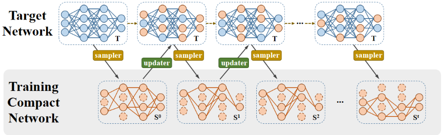
Under the proposed joint search-and-training framework, we have developed a new algorithm for efficiently learning compact networks (refer to Figure 1). In our approach, we alternate between two phases: sampler and updater. In sampling stage, we search for a compact network by weight calculation and thresholding; in the updating stage, the parameters and weights of trained compact network are mapped back to the target network. Meantime, strategies of random perturbation and flexible thresholding are introduced to further improve the efficiency of sampler [Dong and Yang2019c]. After iterative search-and-training, we select the best compact networks and fine-tune them to convergence. We have validated the proposed method on both ResNet and VGGNet and several well-known datasets (CIFAR-10, CIFAR-100 and ImageNet). Our experimental results show that our method can achieve better accuracy results and shorter wall-clock running time when compared to other competing methods.
2 RelatedWorks
Unstructured Network Pruning. Unstructured Pruning methods aim to emphasize the sparseness of filters or channels in large networks. In this way, according to the sparse theory, the pruned network after trimming the sparse terms will have distribution similar to that of large networks without pruning. To optimize the number of neurons in a network, thus the number of parameters, [Zhou et al.2016] incorporates a sparse constraint into the objective function and decimate the number of neurons during the training stage. [Alvarez and Salzmann2016] propose to apply group sparsity regularization on the parameters of the network, where each group is defined to act on a single neuron. Similar to our algorithm, an efficient neural network pruning algorithm is proposed in [Kim et al.2019], which can prune the network in a few minutes. However, due to manual design, this method has no advantage in performance and also relies on the well-trained target network.
Structured Network Pruning. Structured Pruning methods iteratively prune and tune filters or layers in the network to reduce the performance damage of hand-crafted design. A typical pruning paradigm is to first train a large target network, then pruning, and finally fine-tune the compact network. The pruning regulation is to prune the relatively unimportant filters and combine the remaining filters into a new compact network. The mainstream pruning methods focus on how to prune properly under the framework of training before pruning. For example, in [He et al.2019], the redundancy of the filter is determined by introducing geometric median; [He et al.2018a] additionally updates the pruned filter to increase the capacity of the model; [Dong and Yang2019a] applies NAS to search the optimal depth and width of the network; [Liu et al.2019] automatically prune networks by meta-learning. In contrast to previous pruning methods, our method allows direct learning of a compact network through joint search and training in the unpruned network, thereby greatly improving the efficiency.
Lightweight Network Designing. Lightweight Network Designing methods avoid pruning by constructing a simpler network structure than standard networks, while achieving the goal of reducing model parameters and calculations. The most popular lightweight network design methods are MobileNet and ShuffleNet. MobileNet achieves network lightweighting by replacing a standard convolution with a depth-wise separable convolution , which contains a depth-wise convolution and a 1 × 1 convolution. ShuffleNet architecture uses two operations: pointwise group convolution to help reduce computational complexity, and channel shuffle to help information flow. For a given computational complexity budget, ShuffleNet allows more feature maps to be used to help encode more information on small networks.
Network Architecture Search. Network Architecture Search methods aim to find the potentially optimal network structure from hyper-parameterized networks, but usually requires a lot of computing resources and time. Especially for methods based on evolutionary algorithms (EA) [Real et al.2019] and reinforcement learning (RL) [Pham et al.2018, Zoph et al.2018], although those algorithms have made some efforts to improve efficiency. Gradient-based methods [Liu et al.2018a] can effectively reduce the calculation cost. However, in order to make the error back propagation, the number of filters in all candidates is fixed, which also leads to the bloated target network. In [Dong and Yang2019b,Cai et al.2018], the algorithm based on one-shot learning greatly speeds up the training process with parameter sharing, but training a over-parameterized network is still a heavy burden.
3 Efficient Compact Network Learning
3.1 Overview
Different from network pruning, our method does not rely on a pre-trained and over-parametrized model but directly searches and learns a compact network from the scratch. As shown in Figure 1, our approach tackles the problem of joint search-and-training in a coarse-to-fine manner by alternating between two stages: sampler and updater. The sampler searches for compact sub-networks from the target network, while the updater maps the trained sub-networks back to the target network. The best performing sub-network will be further fine-tuned as the final output. Inspired by Monte Carlo and Reinforcement Learning, we count on random perturbation and iterative thresholding to efficiently search a compact network during the sampler stage.
At the starting point, we first need to train the target network coarsely before searching. Similar to previous works [Ye et al.2018], we introduce the concept of setting a flexible threshold for the pruned filter, which requires that the weight can correspond to the importance of the corresponding filter. For this reason, we have added an additional constraint on the weight distribution as a term of training errors in addition to the cross-entropy classification loss. At the initialization, the complete training loss function ℓcoarse to coarsely train the target network T is given by:
where (xi, yi) denote the pair of input/output training data, α is the weight associated with each filter, Ω refers to parameters in the target network T , ‖·‖2 refers to the ℓ2 norm regularization of the weights and λ is the hyper-parameter.
After coarsely training the target network, we continue to iteratively search and obtain a series of compact networks S0 , S1 , . . . , S T as shown by the sampler in Figure 1. These networks will be mapped back to the target network after proper training, which can be interpreted as pruning-based NAS in a coarse-to-fine manner. After the search, we choose a compact network that performs the best on the test set and fine-tune it until reaching convergence. At the core of each sampler is a Threshold network, which plays the role of adapting the thresholds of input layers for network pruning.
3.2 Flexible Pruning via ThresNet
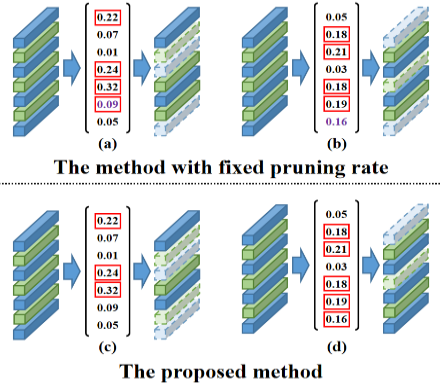
Filters pruning operations are the soul of networking pruning methods because the filter kept at each layer will affect the accuracy of pruned network. Therefore, the pruning operation needs to strike the optimal tradeoff between performance (e.g., accuracy) and cost (e.g., drop rate). Previous filter-wise pruning methods manually control the number of pruned filters. Other filter pruning methods (e.g., [Dong and Yang2019a]) search for the depth and width of a small network and transfer the knowledge from the trained large network to the searched small network. However, the optimality of those filter pruning for a fixed number or drop rate is questionable. For example, when the number of filters selected for each layer is fixed (as shown by the top diagram in Figure 2), it may be the case that some large and significant weights get pruned or some small and insignificant weights get reserved in order to meet the strict pruning rate constraint.
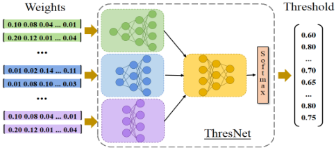
It is conceptually desirable to prune the filters more adaptively - e.g., via thresholding the weights (as shown by the bottom diagram in Figure 2). Inspired by [He et al.2018b] that used reinforcement learning to effectively sample the space of NAS, we propose to train a network called ThresNet to automatically learn the threshold for each layer of the network. We formulate the threshold learning as a sequential decision making process, where an agent - ThresNet parameterized by Φ - can make a sequence of decisions about the threshold βl according to the filter weight αl .
The ThresNet takes αl of each convolutional layer as the input and selects a threshold in the range (e.g., [0.6,0.8] as shown in Figure 3) for each layer as the output decision. This network consists of two parts. The first part is an expansion network decomposed of fully connected layers with varying shape sizes corresponding to different shapes of αl . For example, the varying shape sizes of αl are 16/32/64 respectively in ResNet for the CIFAR dataset. We design a fully connected network with 3 layers/2 layers/1 layer separately in order to make the input shape size (128) consistent. The second part is a shrinking network that reduces the feature dimension from 128 to the shape size in the threshold space and pick the appropriate threshold as the network output.
As the searching process for compact networks goes, the forward propagation loss of each S is first calculated. The opposite of the average of losses in every K episodes is then used as a part of the reward (as in reinforcement learning). In order to avoid finding too large sub-networks, the parameter amount is counted as a restriction and the opposite of it is also used as a part of the reward.
Where R refers to the reward, lavg is the average of losses, γ is the hyper-parameter that balance the two parts of the reward and param(S) denotes the parameter amount. We opt to train the ThresNet using a policy gradient algorithm to learn the policy πΦ with parameters Φ by maximizing the rewards. The policy gradient can be approximated by [Ashok et al.2017]
where Rk is the reward computed at the k-th episode and βl is the threshold agent decided at layer l. Training ThresNet makes it possible to adaptively learn the structure of compact sub-networks, which brings more flexibility to our NAS method. The sequence of thresholds learned by ThreshNet will be exploited to search for a compact sub-network S next.
3.3 Sampler: Search the Compact Subnetwork
Given a target Network T with L layers, we denote all convolution filters in the l-th layer by W l1 ,W l2 , · · · ,W lCl ∈ RCl-1×k×k , where Cl indicates the channel depth of the l-th layer and k represents the kernel size. Therefore, for a given input feature map Il ∈ RCl-1×Hl-1×Wl-1 , the output of the l-th layer Ol can be expressed as:
where ∗ indicates the convolution operation. Note that each channel of the output in this layer can be regarded as the convolutional output of the input and the corresponding convolution filter separately. The goal of network pruning is to
Algorithm 1: Sampler
eliminate unimportant filters for the purpose of reducing the amount of parameters and calculations from the target network. In order to characterize the importance of each convolution filter more directly, we introduce a filter-related weight αl ∈ RCl into those filters and rewrite Eq. (5) as:
Taking filters and their associated weights αl as inputs, sampler outputs a compact subnetwork with pruned filters and updated weights pl . Two optimization strategies are introduced to our sampler: 1) we propose to expand the search space by exploiting the randomness - i.e., filter-related weights are randomly perturbed by uniform noise before calculating the probabilities; 2) we propose to make the thresholds flexible with respect to each layer by leveraging the power of ThreshNet in the previous subsection. When combined together, these two strategies can be interpreted as NAS based on Monte Carlo Search [Dai et al.2019] and Reinforcement Learning [Zoph et al.2018]. The detailed procedure for Sampler is shown in Algorithm 1 where we elaborate on how to choose pruned weights pl and filters W l1,2,...,Fl for the l-th layer based on input weights.
3.4 Joint Search-and-Training
For a searched compact network, the output of each layer can be written as:
where pl is the output of Algorithm 1 and ˆ plc indicates the normalized weights for each layer. By sampling each layer of the network, we can get a compact sub-network S of the
Output: A compact network S
target network T , whose parameters and weights can be expressed by Θ and p, respectively. By feeding these information back to the resampler though the updater as shown in Figure 1, we observe that the search for the most compact subnetwork can be solved iteratively in a coarse-to-fine manner.
Just like the NAS method [Zoph et al.2018], we can update the parameters and weights on the training set Dtrain and validation sets Dvalid successively, which can be formulated as:
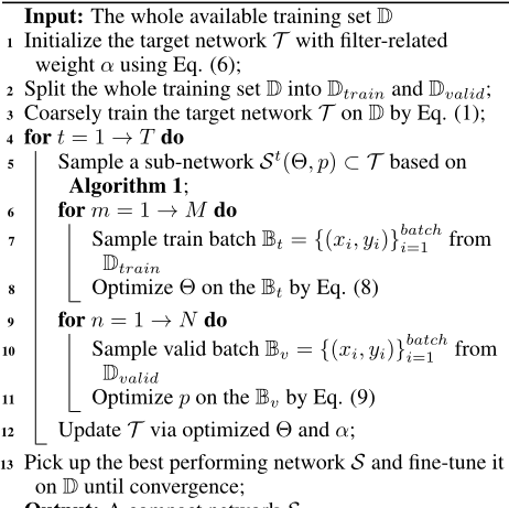
where (xi, yi) indicates the input and corresponding label, ℓtrain and ℓval are the cross-entropy classification loss of the networks, Bt denotes the sampled batches from Dtrain, and so is Bv from Dvalid. After obtaining the optimized Θ and p, we update these parameters back into the target network T . Naturally, in the next search procedure, the sampling of compact subnetworks can benefit from the experience of previous search. In other words, learned knowledge in the NAS space can be iteratively fed back to the sampler, which further improves search efficiency and training performance. In summary, the complete procedure of our joint Search-andTraining Approach is referred to Algorithm 2.
4 Experimental Results
4.1 Experimental Setting
Datasets. We validate our network cropping method on several mainstream datasets. Among them, CIFAR-10 contains 60,000 images categorized into 10 classes. The training set has 5000 images per class, 50,000 images in total. The test set contains 1000 images per class, 10,000 images in total. CIFAR-100 is similar to CIFAR-10. It contains 50,000 training and 10,000 test images, categorized into 100 classes. All images are 32x32 colored ones. ImageNet is a large-scale image classification dataset, containing 1000 classes, 1.28 million training images and 50,000 validation images.
Searching and Training Setup. For searching and training, we randomly extract 80% of the official training images as the training set Dtrain in Algorithm 2, and the rest as the validation set Dval. In our implementation, we search the compact networks with thresholds in the range [0.6,0.65,0.7,0.75,0.8] for each layer.The hyper-parameter λ is set to 0.1, γ is set to 2.0 and all parameters and weights are initialized by kaiming normal in Pytorch. For different dataset, we apply different settings: 1) On CIFAR dataset, we use SGD with the momentum of 0.9 and the weight decay of 0.00005 as optimizer. At the beginning, we train the target network coarsely for 100 epochs with batch size 128. The learning rate is started from 0.1 and reduced by cosine scheduler. Then we search T = 30 compact network, whose parameters are optimized on Dtrain for M (M = 40 for t ⩽ 20, 30 for t > 20) epochs with learning rate of 0.05/0.01, corresponding to different M. And the weights are optimized on Dval for N = 5 epochs with fixed learning rate of 0.001. In the fine-tuning stage, we set batch size of 256, learning rate of 0.01 and optimize the selected compact network until convergence. The number of GPUs we used is consistent with the compared method: for the experiments on CIFAR-10 datasets, we use one NVIDIA Titan XP GPUs for training and searching, and NVIDIA 1080Ti for CIFAR-100. 2) On ImageNet datasets, we optimize the parameters via Adam with weight decay of 0.00001 and the weights via the same SGD as CIFAR. For ResNet model, we coarsely train 40 epochs with an initial learning rate of 0.1 and search T = 20 compact networks. M is set to be 10 with learning rate of 0.001 and N is set to be 2. When finetuning, we set the initial learning rate to 0.001 and divided by 10 every 20 epochs. All experiments on the ImageNet dataset use 4 NVIDIA Titan XP GPUs with batch size of 256.
On CIFAR-10 Dataset. We evaluate our method on ResNet-20,56,110 and 164. We have compared several recently proposed pruning methods with our method, including the soft filter pruning (SFP) [He et al.2018a] method, the method for pruning filters with efficient ConvNet (PFEC) [Li et al.2016], the Geometric Median based filter Pruning (FPGM) [He et al.2019] method and the Transformable Architecture Search (TAS) [Dong and Yang2019a] method. For fairness, the results of other methods were directly borrowed from their papers. As for the consumed time, we calculate the sum of pre-training time, pruning and tuning time, where pruning time is not reported in their paper, so we obtain it through the code and hyper-parameters provided by [He et al.2018a, He et al.2019, Dong and Yang2019a]. In Table 1, We show comparisons in FLOPs, Accuracy and consumed Time in CIFAR-10. With fewer or close FLOPs, our method can achieve nearly 2× the speed increase, and even 0.3 ∼ 1.0% higher accuracy, compared to [Li et al.2016, He et al.2018a, He et al.2019]. Compared with the best performance method [Dong and Yang2019a], our algorithm performs slightly worse on ResNet20 and 56, has lower accuracy on ResNet110 with lower flops, and has better performance on ResNet164. Although our algorithm is short of accuracy of some models compared with [Dong and Yang2019a], it is 3 ∼ 5× faster in speed. Compared with a slight decrease in accuracy, we think lesstraining time is more meaningful to a certain extent. At the same time, you can notice that our baseline is lower than that of [Dong and Yang2019a], which is caused by hardware devices, special training skills andexperienced parameter setting. A more intuitive comparison is "Dropped Acc", on which we arecloser to [Dong and Yang2019a]. Note that only [Dong and Yang2019a] uses the setting of batchsize = 256(Set to 128 in other implementations), which means more GPU occupation. We think that searching the depth and width of the network at the same time is the reason for more searching time and higher accuracy.
| Network | Method | FLOPs | Acc/Drop | Pre-trained | Time Pruning | Finetuning |
|---|---|---|---|---|---|---|
| ResNet20 | SFP [He et al.2018a] | 2.43e7/42.2% | 90.83/1.37↓ | 3h49m | 1h20m | 7 |
| FPGM [He et al.2019] | 2.43e7/42.2% | 91.09/1.11↓ | 3h50m | 3h34m | 7 | |
| TAS [Dong and Yang2019a] | 2.24e7/45.0% | 92.88/0.00↓ | 3 | 7h3m | 1h18m | |
| Ours | 2.27e7/45.1% | 91.95/0.86↓ | 7 | 1h23m | 2h | |
| ResNet56 | PFEC [Li et al.2016] | 9.10e7/27.6% | 91.31/1.59↓ | - | - | - |
| SFP [He et al.2018a] | 5.94e7/52.6% | 93.35/0.24↓ | 3h2m | 1h7m | 7- | |
| FPGM [He et al.2019] | 5.94e7/52.6% | 93.49/0.32↓ | 1h41m | 8h6m | 7 | |
| TAS [Dong and Yang2019a] | 5.95e7/52.7% | 93.69/0.77↓ | 3 | 16h56m | 2h23m | |
| Ours | 6.32e7/49.7% | 93.68/0.73↓ | 7 | 2h20m | 3h6m | |
| Resnet110 | PFEC [Li et al.2016] | 1.66e8/38.6% | 93.44/0.19↓ | - | - | - |
| SFP [He et al.2018a] | 1.50e8/40.8% | 93.86/-0.18↓ | 10h20m | 5h20m | 7 | |
| FPGM [He et al.2019] | 1.21e8/52.3% | 93.85/0.17↓ | 6h3m | 4h20m | 7 | |
| TAS [Dong and Yang2019a] | 1.19e8/53.0% | 94.33/0.64↓ | 3 | 15h11m | 5h45m | |
| Ours | 1.08e8/58.0% | 94.22/0.61↓ | 7 | 3h50m | 3h30m | |
| Resnet164 | TAS [Dong and Yang2019a] | 1.78e8/28.1% | 94.00/1.47↓ | 3 | 47h58m | 6h48m |
| Ours | 1.77e8/28.0% | 94.05/1.22↓ | 7 | 6h50m | 4h50m |
On CIFAR-100 Dataset. In Table 2, we compare the performance of different algorithms on ResNet20, 56, 110 and VGG-16. Because the experimental parameter settings on CIFAR-100 are not provided in [He et al.2019, He et al.2018a], we do not compare time for the sake of fairness. For pruning the ResNet model, our method can still maintain the efficiency of other methods, and the performance is close to [He et al.2018a,He et al.2019] but only slightly worse than [Dong and Yang2019a]. This is because on the CIFAR-100 dataset, there are only 600 training pictures of each category, and only 480 pictures per category in Dtrain, which causes our method to encounter severe under-fitting problems while learning the compact model from scratch. For VGGNet, our method still outperform the sparse based structure selection method(SSS) [Huang and Wang2018] and the genetic algorithm based channel pruning method(GCP) [Hu et al.2018].
| Network | Method | FLOPs/Droped | Acc/Droped | Time |
|---|---|---|---|---|
| SFP [He et al.2018a] | 2.43e7/42.2% | 64.37/3.25↓ | - | |
| ResNet20 | FPGM [He et al.2019] | 2.43e7/42.2% | 66.86/0.86↓ | - |
| TAS [Dong and Yang2019a] | 2.24e7/45.0% | 68.90/-0.21↓ | 8.3h | |
| Ours(fixed rate) | 2.05e7/49.7% | 67.28/1.31↓ | 5.5h | |
| Ours | 2.27e7/45.9% | 66.48/2.11↓ | 5.0h | |
| SFP [He et al.2018a] | 5.94e7/52.6% | 68.79/2.61↓ | - | |
| ResNet56 | FPGM [He et al.2019] | 5.94e7/52.6% | 69.66/1.75↓ | - |
| TAS [Dong and Yang2019a] | 6.12e7/51.3% | 72.25/0.93↓ | 20.0h | |
| Ours(fixed rate) | 6.72e7/51.1% | 70.07/2.86↓ | 11.0h | |
| Ours | 6.72e7/51.1% | 70.63/2.26↓ | 11.5h | |
| SFP [He et al.2018a] | 1.21e8/52.3% | 71.28/2.86↓ | - | |
| Resnet110 | FPGM [He et al.2019] | 1.21e8/52.6% | 72.55/1.59↓ | - |
| TAS [Dong and Yang2019a] | 1.20e8/51.3% | 73.16/1.90↓ | 34.5h | |
| Ours(fixed rate) | 1.08e8/58.0% | 71.69/2.73↓ | 13.0h | |
| Ours | 1.08e8/58.0% | 72.26/2.16↓ | 9.5h | |
| GCP [Hu et al.2018] | 3.82e8/39.1% | 72.01/1.18↓ | - | |
| VGG-16 | SSS [Huang andWang2018] | 3.08e8/50.6% | 72.95/0.24↓ | - |
| Ours | 3.22e8/48.4% | 74.63/1.12↓ | 4.5h |
| Method | FLOPs/Droped | Acc/Droped | Time | |
|---|---|---|---|---|
| Top-1 | Top-5 | |||
| SFP [He et al.2018a] | 2.38e9/41.8% | 74.61/1.54↓ | 92.06/0.81↓ | 130h |
| FPGM [He et al.2019] | 2.36e9/42.2% | 75.50/0.65↓ | 92.63/0.21↓ | 112h |
| TAS [Dong and Yang2019a] | 2.31e9/43.5% | 76.20/1.26↓ | 93.07/0.48↓ | 170h |
| Ours | 2.25e9/44.9% | 75.51/1.01↓ | 92.43/0.66↓ | 90h |
On ImageNet Dataset. In Table 3, we use 4 NVIDIA 2080Ti GPUs to validate our method on the ResNet-50 model. Compared to the other state-of-the-art algorithm, we still show competitive results. For example, we can prune ResNet-50 in 88 hours, and the prunned network can achieve 75.51%/92.43% accuracy. The training time of the complete ResNet-50 model is nearly 80 hours, which means that we can complete the entire search algorithm in the same time as other algorithms training unpruned models.
4.2 Ablation Study
In order to show the effect of flexible pruning, we implemented a baseline version of the proposed method, that is, pruning with a manually determined fixed crop rate (the "fixed rate" method in Table 2). We calculate the appropriate pruning rate based on the implementation based on flexible pruning and apply it to each layer of the network (as shown top of Figure 2). We verified ResNet-20,56 and 110 on the CIFAR-100 dataset. Compared with a fixed pruning rate, the flexible pruning method can effectively speed up the search and improve the performance of the searched network.For example, when cropping resnet56, our method based on flexible pruning achieved a 0.57% performance improvement in less time than the fixed cropping method. Note that we are just training a simple fully connected network as a ThresNet with a basic reinforcement learning strategy, so the performance of our algorithm can also be improved by using more powerful networks and more effective reinforcement learning methods.
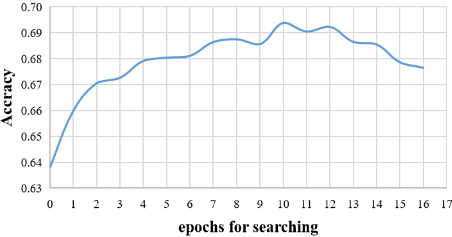
A very important part of our approach is to select the best performing sub-networks for fine-tuning at the end of the training-search process, so to better illustrate the search-andtraining procedure, we provide the performance of all sampled networks. In fact, after the search-and-training procedure (corresponding to lines 4-12 in Algorithm 2), we actually get some pretty good but not well-trained sub-networks. Then, as described in Algorithm 2, line 13, we select and optimize the network with the best performance. In our method, it is unnecessary to ensure that every sub-network is welltrained after search-and-training procedure. And there are two reasons: first, training every sampled sub-network to convergence will greatly improve the time cost and calculation cost of the algorithm; second, in the process of searching, a well-trained sub-network will lead to the reduction of search space, which limits the sub-network to be searched later. Therefore, the bias towards the last sampled network that you're worried about won't happen either. In fact, in our experiments, the best performing sub-network usually appeared in the middle of the training epochs, as shown in Figure 4
5 Conclusion
In this paper, we propose a new joint search and training method designed to learn a compact network directly from scratch. First, we propose to iteratively sample and update compact networks to approximate the target network. Unlike most previous methods, we do not follow the rule of pruning-after-training, but jointly search and train to learn compact networks directly from unclipped networks. Secondly, we have developed a flexible pruning method that flexibly adjusts the weight and size of each layer by learning a set of filter-related weights. For this part, we propose to optimize the ThresNet by reinforcement learning. On some benchmark datasets and network architectures, our proposed method achieves transcendental efficiency improvements while achieving competitive classification accuracy.
Acknowledgements
This work was supported in part by the National Key RD Program of China under Grant 2018AAA0101400 and the Natural Science Foundation of China under Grant 61991451, Grant 61632019, Grant 61621005, and Grant 61836008.
@inproceedings{ijcai2020p358,
  title     = {Beyond Network Pruning: a Joint Search-and-Training Approach},
  author    = {Lu, Xiaotong and Huang, Han and Dong, Weisheng and Li, Xin and Shi, Guangming},
  booktitle = {Proceedings of the Twenty-Ninth International Joint Conference on
               Artificial Intelligence, {IJCAI-20}},
  publisher = {International Joint Conferences on Artificial Intelligence Organization},
  editor    = {Christian Bessiere},
  pages     = {2583--2590},
  year      = {2020},
  month     = {7},
  note      = {Main track},
  doi       = {10.24963/ijcai.2020/358},
  url       = {https://doi.org/10.24963/ijcai.2020/358},
}
TY - CPAPER TI - Beyond Network Pruning: a Joint Search-and-Training Approach AU - Lu, Xiaotong AU - Huang, Han AU - Dong, Weisheng AU - Li, Xin AU - Shi, Guangming T2 - Proceedings of the Twenty-Ninth International Joint Conference on Artificial Intelligence, IJCAI-20 PB - International Joint Conferences on Artificial Intelligence Organization PY - 2020 SP - 2583 EP - 2590 DO - 10.24963/ijcai.2020/358 UR - https://doi.org/10.24963/ijcai.2020/358 ER -Copied
Machine-readable versions of this paper, for tools and AI agents:





