
Learning from Few Positives: a Provably Accurate Metric Learning Algorithm to Deal with Imbalanced Data
Proceedings of the Twenty-Ninth International Joint Conference on Artificial Intelligence. Main track. Pages 2155-2161.
https://doi.org/10.24963/ijcai.2020/298
Keywords
- Machine Learning Applications: Applications of Supervised Learning
- Machine Learning: Classification
Abstract
Learning from imbalanced data, where the positive examples are very scarce, remains a challenging task from both a theoretical and algorithmic perspective. In this paper, we address this problem using a metric learning strategy. Unlike the state-of-the-art methods, our algorithm MLFP, for Metric Learning from Few Positives, learns a new representation that is used only when a test query is compared to a minority training example. From a geometric perspective, it artificially brings positive examples closer to the query without changing the distances to the negative (majority class) data. This strategy allows us to expand the decision boundaries around the positives, yielding a better F-Measure, a criterion which is suited to deal with imbalanced scenarios. Beyond the algorithmic contribution provided by MLFP, our paper presents generalization guarantees on the false positive and false negative rates. Extensive experiments conducted on several imbalanced datasets show the effectiveness of our method.
- [Abdallah et al., 2016] Aisha Abdallah, Mohd Aizaini Maarof, and Anazida Zainal. Fraud detection system: A survey. Journal of Network and Computer Applications, 68:90-113, 2016.
- [Aggarwal, 2017] Charu C. Aggarwal. Outlier Analysis. Springer International Publishing, 2017.
- [Bellet et al., 2013] Aurélien Bellet, Amaury Habrard, and Marc Sebban. A survey on metric learning for feature vec- tors and structured data. CoRR, abs/1306.6709, 2013.
- [Bellet et al., 2015] Aurélien Bellet, Amaury Habrard, and Marc Sebban. Metric Learning. Synthesis Lectures on Artificial Intelligence and Machine Learning. Morgan & Claypool Publishers, 2015.
- [Bousquet and Elisseeff, 2002] Olivier Bousquet and André Elisseeff. Stability and generalization. Journal of machine learning research, 2(Mar):499-526, 2002.
- [Davis et al., 2007] Jason V. Davis, Brian Kulis, Prateek Jain, Suvrit Sra, and Inderjit S. Dhillon. Information- theoretic metric learning. In Proceedings of the 24th inter- national conference on Machine learning, pages 209-216. ACM, 2007.
- [Ding et al., 2018] Shuya Ding, Bilal Mirza, Zhiping Lin, Ji- uwen Cao, Xiaoping Lai, Tam V. Nguyen, and Jose Sepul- veda. Kernel based online learning for imbalance multi- class classification. Neurocomputing, 277:139-148, 2018.
- [Dumpala et al., 2018] Sri Harsha Dumpala, Rupayan Chakraborty, and Sunil Kumar Kopparapu. A novel data representation for effective learning in class imbalanced scenarios. In Proceedings of the 27th International Joint Conference on Artificial Intelligence, pages 2100-2106, 7 2018.
- [Feng et al., 2018] Lin Feng, Huibing Wang, Bo Jin, Hao- hao Li, Mingliang Xue, and Le Wang. Learning a dis- tance metric by balancing kl-divergence for imbalanced datasets. IEEE Transactions on Systems, Man, and Cy- bernetics: Systems, PP:1-12, 01 2018.
- [Frery et al., 2018] Jordan Frery, Amaury Habrard, Marc Sebban, and Liyun He-Guelton. Non-linear gradient boosting for class-imbalance learning. In 2nd Interna- tional Workshop on Learning with Imbalanced Domains: Theory and Applications, pages 38-51, 2018.
- [Gautheron et al., 2019] Léo Gautheron, Emilie Morvant, Amaury Habrard, and Marc Sebban. Metric learning from imbalanced data. In arXiv. 1909.01651, 2019.
- [Huang et al., 2016] Chen Huang, Yining Li, Chen Change Loy, and Xiaoou Tang. Learning deep rep- resentation for imbalanced classification. In Proceedings of the IEEE conference on computer vision and pattern recognition, pages 5375-5384, 2016.
- [Khan et al., 2017] Salman H. Khan, Munawar Hayat, Mo- hammed Bennamoun, Ferdous A. Sohel, and Roberto Togneri. Cost-sensitive learning of deep feature represen- tations from imbalanced data. IEEE transactions on neural networks and learning systems, 29(8):3573-3587, 2017.
- [Kulis and others, 2013] Brian Kulis et al. Metric learning: A survey. Foundations and Trends R in Machine Learn- ing, 5(4):287-364, 2013.
- [Mathew et al., 2015] Josey Mathew, Ming Luo, Chee Khi- ang Pang, and Hian Leng Chan. Kernel-based smote for svm classification of imbalanced datasets. In IECON 2015-41st Annual Conference of the IEEE Industrial Elec- tronics Society, pages 001127-001132. IEEE, 2015.
- [Pérez-Ortiz et al., 2019] María Pérez-Ortiz, Peter Tiño, Rafal Mantiuk, and César Hervás-Martínez. Exploit- ing synthetically generated data with semi-supervised learning for small and imbalanced datasets. CoRR, abs/1903.10022, 2019.
- [Rijsbergen, 1979] Cornelis J. Van Rijsbergen. Information Retrieval. 1979.
- [Schiller, 2006] Jörg Schiller. The impact of insurance fraud detection systems. Journal of Risk and Insurance, 73(3):421-438, 2006.
- [Sharma et al., 2018] Shiven Sharma, Colin Bellinger, Bar- tosz Krawczyk, Osmar R. Zaïane, and Nathalie Japkow- icz. Synthetic oversampling with the majority class: A new perspective on handling extreme imbalance. IEEE In- ternational Conference on Data Mining, pages 447-456, 2018.
- [Wang et al., 2018] Nan Wang, Xibin Zhao, Yu Jiang, Yue Gao, and KLISS BNRist. Iterative metric learning for imbalance data classification. In 27th International Joint Conference on Artificial Intelligence, pages 2805-2811, 2018. IJCAI
- [Weinberger and Saul, 2009] Kilian Q. Weinberger and Lawrence K. Saul. Distance metric learning for large mar- gin nearest neighbor classification. Journal of Machine Learning Research, 10(Feb):207-244, 2009.
- [Wu et al., 2017] Fei Wu, Xiao-Yuan Jing, Shiguang Shan, Wangmeng Zuo, and Jing-Yu Yang. Multiset feature learn- ing for highly imbalanced data classification. In Proceed- ings of the Thirty-First AAAI Conference on Artificial In- telligence, AAAI'17, page 1583-1589. AAAI Press, 2017.
- [Zantedeschi et al., 2016] Valentina Zantedeschi, Rémi Emonet, and Marc Sebban. Metric learning as convex combinations of local models with generalization guaran- tees. In Proceedings of the IEEE Conference on Computer Vision and Pattern Recognition, pages 1478-1486, 2016.
- [Zhang et al., 2019] Xiaogang Zhang, Dingxiang Wang, Yi- cong Zhou, Hua Chen, Fanyong Cheng, and Min Liu. Ker- nel modified optimal margin distribution machine for im- balanced data classification. Pattern Recognition Letters, 125:325-332, 2019.
References were extracted automatically from the PDF and may contain errors.
Full text extracted automatically from the PDF; figures, tables and equations may differ. The PDF is the version of record.
1 Introduction
Fraud detection in bank or insurance applications [Abdallah et al., 2016; Schiller, 2006], and anomaly identification for medical diagnosis [Aggarwal, 2017] are some societal challenges requiring to address the problem of learning from highly imbalanced data. When dealing with such a setting, one has to face two major issues: (i) the scarcity of the class of interest, only composed of a few positive data, which limits the efficiency of standard margin-based loss functions; (ii) the scattering of positive examples in the total mass of the training data, which makes the estimation of local densities much more complicated than in balanced scenarios. Several solutions have been proposed in the literature to address these two problems. Most of them consist in applying sampling strategies which aim to balance the dataset by reducing the number of negative examples and/or creating new synthetic positive data [Sharma et al., 2018; P´erez-Ortiz et al., 2019]. On the other hand, one can resort to cost-sensitive algorithms [Khan et al., 2017] which assign a weight to each class (or even to each example) so that the classifier can focus better on the minority class. Other strategies include the use of ensemble methods [Wu et al., 2017; Frery et al., 2018] or the specific adaptation of existing approaches such as deep learning [Huang et al., 2016; Dumpala et al., 2018] or kernel methods [Mathew et al., 2015; Ding et al., 2018; Zhang et al., 2019].
In this paper, we address the problem of learning from imbalanced data from a metric learning perspective [Bellet et al., 2013; Kulis and others, 2013]. Learning a metric specifically designed for the application at hand may present several advantages in the context of imbalanced datasets: (i) the metric can be learned under semantic constraints allowing us to expand the decision boundaries around the positives; (ii) this framework enables to design optimization problems based on the geometry of the data without suffering from the issues of standard accuracy-based loss functions (e.g., hinge loss for SVMs, exponential loss for boosting, logistic loss for logistic regression); (iii) metric learning is a nice setting to derive theoretical guarantees on the learned transformation [Bellet et al., 2015]. Surprisingly, despite these interesting features, metric learning has not received much attention to address the problem of learning from imbalanced data (see, e.g., the recent papers [Feng et al., 2018], [Wang et al., 2018] and [Gautheron et al., 2019]). The goal of this paper is to bridge this gap from both an algorithmic and a theoretical perspective. As illustrated in Figure 1, we propose the algorithm MLFP that optimizes a linear transformation (via a Positive Semi Definite (PSD) matrix M of a Mahalanobis distance) only when a test query is compared to a minority training example. A single metric M is learned for the whole space taking the geometry of the data into account. Unlike the standard metric learning algorithms (see, e.g., LMNN [Weinberger and Saul, 2009] or ITML [Davis et al., 2007]), our method boils down to artificially bringing positive examples closer to the query without challenging the features of the negatives. This has a direct impact on the decision boundaries around the positives allowing us to capture more examples of the class of interest yielding a better F-Measure (see Section 3 for a formal definition). By using the uniform stability framework, we derive theoretical guarantees on the learned matrix M showing the actual capability of MLFP to control the false positive and false negative rates.
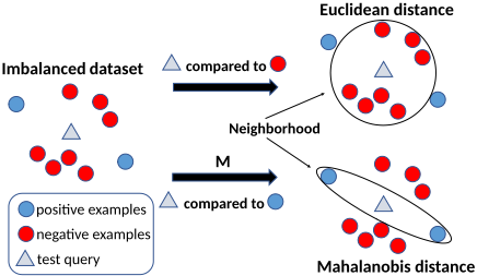
The paper is organized as follows. In Section 2, we report some related work on metric learning for imbalanced data classification. Section 3 is dedicated to the presentation of our metric learning algorithm MLFP. Section 4 presents a theoretical analysis using the uniform stability framework and Section 5 illustrates the performance of MLFP compared to state-of-the-art algorithms.
2 RelatedWork
Most of the metric learning algorithms (see [Bellet et al., 2013; Kulis and others, 2013] for a survey) are based on the optimization of the Mahalanobis distance between two points xi and xj ∈ Rq :
where M is a q × q Positive Semi Definite matrix. One can express M as LT L where L is a r × q matrix where r is the rank of M. Thus, this distance can be seen as the Euclidean distance in a new feature space Lx.
A well-known representative of this family of algorithms is the Large Margin Nearest Neighbor (LMNN) [Weinberger and Saul, 2009]. For each example of a training set of size m, the learned metric M aims to bring closer the neighbors of the same class (called target neighbors) while pushing away the examples of other classes (the impostors). This algorithm has been shown to be very efficient and to scale well with large datasets. However, it is worth noticing that LMNN is not designed to take into account some imbalance in the data. Indeed, the similarity constraints constructed from pairs of examples of the same class do not make any difference between the positive and negative examples. Therefore, in imbalanced scenarios, LMNN, as the other state-of-the-art methods, is prone to focus on the majority class and thus is subject to miss the positive examples.
The first attempts to address the problem of learning a metric from imbalanced datasets have been proposed very recently. [Wang et al., 2018] introduce an iterative metric learning algorithm (IML) that aims to define a stable neighborhood used to predict the label of a new test data. The method repeats two main steps: (i) the learning of a linear transformation, e.g., by using LMNN, and (ii) a training sample selection given a test example. The procedure is repeated until stabilization of the neighborhood. By repeating the process several times, IML is able to locally separate positives from negatives. However, the main issue comes from the algorithmic complexity of the method, which requires to apply LMNN and to update the pairs used for the training process at each iteration. Another approach to learn metrics from imbalanced datasets has been recently proposed [Gautheron et al., 2019]. In their Imbalanced Metric Learning algorithm (ImbML), the authors take into account the nature of the pairwise constraints by using two different sub-losses, one for each label, weighted according to the number of positive and negative examples respectively. This intuitive and natural way to proceed prevents the algorithm from favoring the majority class. However, we will see that applying the learned metric M to all examples is not necessary, focusing only on the minority class appears to be much more efficient and allows us notably to better control the false negatives. Finally, [Feng et al., 2018] introduce DMBK for Distance Metric by Balancing KL-divergence. This algorithm resorts to the KL-divergence to represent normalized between-class divergences. Combined with a geometric mean, DMBK is able to make these divergences balanced. Note that this method makes sense in the multi-class setting, but is meaningless for addressing binary problems, due to the use of the normalization while computing the KL-divergence.
Beyond the algorithmic limitations of the previous state-ofthe-art algorithms, note that none of them comes with guarantees on the classification error. In this paper, we address this problem by studying the capability of MLFP to optimize a metric M which provides a good compromise between (i) expanding the decision boundaries around the positives which enables to reduce the false negative rate at test time (one of the main issues faced in imbalanced learning); (ii) controlling this expansion to prevent the algorithm from detecting too many false alarms, represented by the false positive rate. The theoretical results take the form of guarantees on the learned metric using the uniform stability framework [Bousquet and Elisseeff, 2002] which measures the stability of the output of the algorithm when the training set is subject to slight changes.
3 Metric Learning for Imbalanced Data
In this section, we present our algorithm MLFP, for Metric Learning from Few Positives. In the following, we denote by S = {zi = (xi, yi)}mi=1 the set of m training examples drawn i.i.d. from an unknown joint distribution D over X×Y, where xi ∈ X (here X = Rq ) is a feature vector and yi ∈ Y (here Y = {-1, +1}) corresponds to its associated label. The label +1 is used to denote the positive or the minority class. We further note S = S+ ∪ S- with S+ the set of m+ positive examples and S- the set of m- negative examples, such that m = m+ + m-.
3.1 ProblemFormulation
In our approach, we use the Euclidean distance when comparing a query point to a majority-class example. The originality comes from the use of an optimized Mahalanobis distance when comparing a query to a minority-class sample. The objective of this strategy is to formulate a metric learning problem leading to a classifier (a kNN here) which is accurate on both classes even in an imbalanced scenario.
In order to avoid the pitfall of classic metric learning algorithms that are prone to focus on the majority class, we propose to give more importance to the minority class composed of the positive instances. Our algorithmMLFP tries to control the false positive (FP) and false negative (FN) rates thanks to the following constrained optimization problem:
where S+ is the set of PSD matrices, λmax(M) is the largest eigenvalue of the PSD matrix M, ℓFN and ℓFP are defined by:
where [a]+ = max(0, a), α is the positive rate m+ m and µ‖M- I‖2F is a regularization term which penalizes a large deviation from the Euclidean distance. The hyper-parameter c controls the margin we want to preserve between pairs of dissimilar examples according to the Euclidean space and the learned one.
Problem (1) is composed of two terms where triplets are involved. Unlike standard metric learning algorithms, our method takes into account both the Euclidean distance d and the metric learned dM. More precisely: the first term ℓFN aims to gather the minority class examples with respect to the learned metric such that the distance between two positives (using M) is less than the distance to a negative example (using the Euclidean distance). This subloss can be seen as a way to prevent the model from generating false negatives (FN). The second term ℓFP works in a similar manner. The only difference lies in the fact that the query xi is a negative example. Thus, we learn M such that the positive queries xk are not bringing too close to xi, i.e. the Euclidean distance between two negatives xi and xj (with respect to the Euclidean distance) is lower than the distance between xi and xk (with respect to M). This subloss can be seen as a way to prevent the model from generating false positives (FP).
Both FN and FP are important terms to optimize measures that are more suited to deal with imbalanced settings, such as the F-Measure [Rijsbergen, 1979] defined as follows:
Minimizing the F-Measure boils down to finding a good trade-off between FP and FN. However, in a highly imbalanced setting, where m+ is very low, missing only a few positives leads to a dramatic decrease of the F-Measure. That is why we constrain the largest eigenvalue λmax(M) to be lower than 1, so that the learned matrixM aims to pay more attention to the positive class. In the next section, we provide a formal explanation of its use.
3.2 On the Impact of the Constraint
We study the impact of the λmax(M) value on both FN and FP and, thus the influence of the constraint of our optimization problem.
Proposition 1. Let P[FNM(x)] (resp. P[FPM(x)]) be the probability of a positive query (resp. a negative query) x of being a false negative (resp. a false positive) using the 1-NN algorithm with the learned matrix M and P[FN(x)] (resp. P[FP(x)]) the same probability using the Euclidean distance.
Then, if λmax(M) ≤ 1, we have:
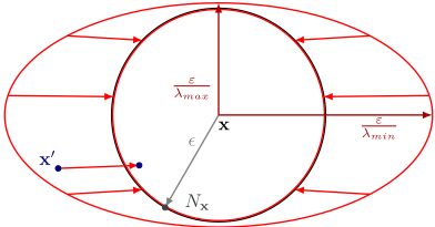
Sketch of proof. Let ε be the distance from x to its nearest neighbor Nx. The example x is a false negative if Nx ∈ S-, that is, all positives x′ ∈ S+ are outside an ellipsoid Eε,M-1 (x), defined by ε and M. Therefore, we have:
When the Euclidean distance is used, we deal with a standard sphere Sε of radius ε, and we get:
Having λmax(M) ≤ 1 implies Eq. (2) ≤ Eq. (3). Indeed λmax(M) ≤ 1 implies that the sphere Sε is included in the ellipsoid Eε,M-1 as illustrated in Figure 2. By this choice, we expand the decision boundaries around positives and thus capture more minority class examples. Using a similar scheme, we can prove the second inequality of Proposition 1. When x is negative and Nx ∈ S+, we have
and
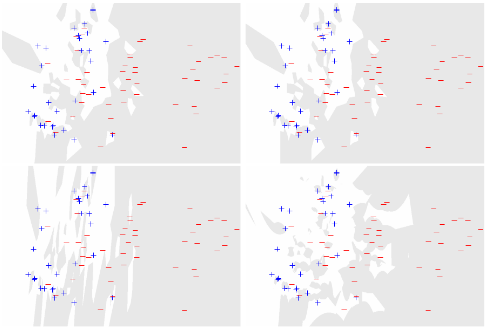
From Equations (2) and (4), we can note that they are both exponentially decreasing w.r.t. to the number of positives and negatives respectively. However, in imbalanced scenarios, the number of negatives is supposed to be much higher than the number of positives. Thus, the probability of having a false positive is decreasing faster than the probability of having a false negative. We then choose to learn a matrix M under the constraint λmax(M) ≤ 1, so that our algorithm will focus first on reducing FN. An illustration of the impact of this constraint in terms of decision boundaries is shown in Figure 3. The experiments in Section 5 will confirm that the use of this constraint is very relevant from an F-Measure perspective and is able to reduce the number of FN at test time.
4 Theoretical Analysis
In this section, we provide generalization guarantees about the learned metric M using the uniform stability framework [Bousquet and Elisseeff, 2002] adapted to metric learning [Bellet et al., 2015]. Then, we use this result to derive classification guarantees over a 1-Nearest Neighbor (1NN) classifier making use of this metric. Note that the whole study is conducted under the constraint λmax(M) ≤ 1 as used in Problem (1).
First, we denote by ℓ the weighted combination of ℓFN and ℓFP as defined in Problem (1) and FS the objective function to optimize over the training set S = {zi}mi=1 . We have
Let RS be the associated empirical risk over S defined as
and R be the corresponding expected true risk defined as
The last equality is due to the i.i.d. aspect of the expectation. We also suppose that for all x, we have ‖x‖ ≤ K.
4.1 Uniform Stability
Intuitively, an algorithm is stable if its output, in terms of loss, does not change significantly under a small modification of the training sample. The supremum of this change must be bounded in O(1/m).
Definition 1. A learning algorithmA has a uniform stability in κm with respect to a loss function ℓ and parameter set θ, with κ a positive constant if:
where S is a learning sample of size m, Z = (z1, z2, z3) = ((x1, y1), (x2, y2), (x3, y3)) is a triplet of labeled examples, θS the model parameters learned from S, θSi the model parameters learned from the sample Si obtained by replacing the ith example zi from S by another example z′i independent from S and drawn from D. Finally, ℓ(θS,Z) is the loss suffered at Z.
In this definition, Si represents the notion of small modification of the training sample. The next definition aims to study the evolution of the loss function according to the considered triplets Z and Z ′ .
Definition 2. A loss function ℓ is said to be γ-admissible, w.r.t. the distance metric M if (i) it is convex w.r.t. its first argument and (ii) if the following condition holds:
where Z = (zi, zj , zk) and Z ′ = (z′i , z′j , z′k ) are two triplets from a sample S and drawn from D.
From the two above definitions, we can state the following generalization bound.
Theorem 1. Let δ > 0 and m > 2. Let S be a sample of m randomly selected training examples. Let M be the matrix learned from Problem (1) which has a uniform stability in κm . The loss function ℓ as defined above is γ-admissible. With probability 1 - δ, the following bound on the true risk R of ℓ holds:
where
The derived bound provides guarantees on the generalization performances of the learned metric on the distribution D w.r.t. to the loss ℓ. We now make use of this bound to provide classification guarantees of a 1NN making use of the learned metric M.
4.2 Classification Guarantees
We derive here generalization guarantees on the FP and FN rates for a 1NN classifier making use of the metric M learned by MLFP. Let S be the learning sample of size m used by a nearest-neighbor classifier. Let us define the empirical risks for FP and FN:
where xp, xn ∈ S are respectively the nearest positive and negative neighbors of x in S. Symmetrically, we have:
We consider then the expected true risks averaged over all the training samples of size m:
We can now introduce our main result.
Theorem 2. Let δ > 0 and m > 0. Let S be a training sample of size m i.i.d. from a distribution D, z a new instance i.i.d. from D, and let M be the learned matrix from Problem (1) which has a uniform stability in κm with respect to the loss ℓ. Considering that the loss function ℓ is γ-admissible, let us denote by RS its empirical risk. With probability 1-δ, we have the following bounds for the FP and FN rates:
By comparing these two bounds, one can observe that when the class imbalance becomes important, i.e. when α takes a low value, the guarantees on the FN rate become better than the guarantees on FP. This result provides a theoretical confirmation that our approach - thanks to the constraint λmax(M) ≤ 1 - is able to focus more on reducing FN. An illustration of this phenomenon will be shown in the next section.
.
5 Experiments
In this section, we compare MLFP to other metric learning algorithms, focusing on (highly) imbalanced datasets. For all experiments, we use a 3-Nearest Neighbor classifier as done in both [Weinberger and Saul, 2009] and [Wang et al., 2018]. Note that the source code allowing the interested reader to reproduce these experiments is available 1 .
5.1 Experimental Setup
We use several public datasets from the UCI 2 and KEEL 3 repositories. These datasets are diverse in terms of imbalance ratio (IR, number of majority examples per positive example), dimension, number of examples, as shown in Table 1. All the datasets are standardized by substracting the mean and dividing by the standard deviation.
We use the F-Measure as the performance criterion to compare the different methods.
Furthermore, 80% of the dataset is randomly selected in order to train the model and 20% to test it. The different hyperparameters are tuned with a 10-fold-cross-validation over the training set. The sampling of the test set is repeated 5 times and we report the average results in terms of F -Measure (F1).
For our MLFP method, the hyper-parameters µ for the regularization and c for the margin are both tuned in the range [0, 1], using a Bayesian optimization with 400 calls. The Bayesian optimization is done with the Scikit-Optimize library 4 . As the matrix M can be expressed as LT L (Cholesky decomposition), we directly learn a diagonal matrix L. Since we are not particularly interested, in this paper, in low rank matrices, we do not impose any constraint on the dimension of L. At each iteration of the optimization process, the spectral radius of the matrix L is constrained to be less than one so that M= LT L has its largest value less than one.
We compare MLFP with several methods: The 3-Nearest Neighbor algorithm (3NN), as a baseline. LMNN, where the hyper-parameter µ, which controls the trade-off between the two parts of the loss (see [Weinberger and Saul, 2009] for more details), is tuned in [0, 1] using a Bayesian optimization with 20 calls. ITML [Davis et al., 2007]. IML [Wang et al., 2018] where we select 5k points for the sampling selection and we also tune the hyper-parameter of the LMNN algorithm in [0, 1]. We used 0.8 for the ratio of matching as suggested in the paper. ImbML [Gautheron et al., 2019] where the parameter m is tuned in {1, 10, 100, 1000, 10000}, the parameter λ in {0, 0.01, 0.1, 1, 10} and the parameter a in [0, 1]. We also use a Bayesian optimization with 400 calls.
5.2 Results
The main results are reported in Table 1. Unsurprisingly, all metric learning methods perform better than a 3NN. Furthermore, in terms of F-Measure, those which were designed to deal with imbalanced scenarios perform better than LMNN or ITML. However, the most competitive method is MLFP:
1 https://github.com/RemiViola/MLFP
2 https://archive.ics.uci.edu/ml/datasets.html
3 https://sci2s.ugr.es/keel/datasets.php
4 https://scikit-optimize.github.io/
| DATASETS | SIZE | DIM | IR | 3NN | LMNN | ITML | IML | IMBML | MLFP (OURS) |
|---|---|---|---|---|---|---|---|---|---|
| BALANCE | 625 | 4 | 1.2 | 0.880 ± 0.018 | 0.874 ± 0.019 | 0.931 ± 0.032 | 0.886 ± 0.029 | 0.960 ± 0.019 | 0.874 ± 0.003 |
| AUTOMPG | 392 | 7 | 1.7 | 0.780 ± 0.054 | 0.792 ± 0.031 | 0.801 ± 0.018 | 0.785 ± 0.021 | 0.790 ± 0.044 | 0.805 ± 0.021 |
| IONOSPHERE | 351 | 34, | 1.8 | 0.745 ± 0.015 | 0.803 ± 0.049 | 0.831 ± 0.054 | 0.823 ± 0.044 | 0.786 ± 0.053 | 0.923 ± 0.026 |
| PIMA | 768 | 8 | 1.9 | 0.601 ± 0.042 | 0.591 ± 0.037 | 0.583 ± 0.022 | 0.591 ± 0.037 | 0.575 ± 0.026 | 0.635 ± 0.032 |
| WINE | 178 | 13 | 2 | 0.968 ± 0.016 | 0.992 ± 0.016 | 0.992 ± 0.016 | 0.992 ± 0.016 | 0.992 ± 0.016 | 0.961 ± 0.041 |
| GLASS | 214 | 9 | 2.1 | 0.735 ± 0.049 | 0.710 ± 0.064 | 0.759 ± 0.051 | 0.710 ± 0.064 | 0.716 ± 0.043 | 0.747 ± 0.034 |
| GERMAN | 1000 | 23 | 2.3 | 0.407 ± 0.049 | 0.358 ± 0.029 | 0.430 ± 0.073 | 0.352 ± 0.029 | 0.388 ± 0.043 | 0.511 ± 0.006 |
| VEHICLE | 846 | 18 | 3.3 | 0.850 ± 0.045 | 0.928 ± 0.024 | 0.931 ± 0.019 | 0.933 ± 0.026 | 0.937 ± 0.014 | 0.859 ± 0.037 |
| HAYES | 132 | 4 | 3.4 | 0.581 ± 0.210 | 0.824 ± 0.089 | 0.829 ± 0.071 | 0.824 ± 0.089 | 0.908 ± 0.083 | 0.930 ± 0.109 |
| SEGMENTATION | 2310 | 19 | 6 | 0.882 ± 0.031 | 0.888 ± 0.011 | 0.866 ± 0.029 | 0.895 ± 0.020 | 0.909 ± 0.028 | 0.882 ± 0.024 |
| ABALONE8 | 4177 | 10 | 6.4 | 0.223 ± 0.025 | 0.220 ± 0.040 | 0.213 ± 0.025 | 0.228 ± 0.021 | 0.200 ± 0.023 | 0.336 ± 0.018 |
| YEAST3 | 1484 | 8 | 8.1 | 0.719 ± 0.028 | 0.734 ± 0.020 | 0.742 ± 0.034 | 0.717 ± 0.032 | 0.723 ± 0.023 | 0.725 ± 0.022 |
| PAGEBLOCKS | 5473 | 10 | 8.8 | 0.855 ± 0.027 | 0.844 ± 0.027 | 0.850 ± 0.023 | 0.842 ± 0.027 | 0.865 ± 0.021 | 0.860 ± 0.022 |
| SATIMAGE | 6435 | 36 | 9.3 | 0.688 ± 0.034 | 0.707 ± 0.038 | 0.710 ± 0.024 | 0.710 ± 0.039 | 0.731 ± 0.030 | 0.697 ± 0.030 |
| LIBRAS | 360 | 90 | 14 | 0.694 ± 0.188 | 0.725 ± 0.105 | 0.722 ± 0.204 | 0.690 ± 0.120 | 0.729 ± 0.157 | 0.694 ± 0.066 |
| REDWINEQUALITY4 | 1599 | 11 | 29.2 | 0.062 ± 0.075 | 0.057 ± 0.114 | 0.027 ± 0.053 | 0.000 ± 0.000 | 0.031 ± 0.062 | 0.083 ± 0.039 |
| YEAST6 | 1484 | 8 | 41.4 | 0.560 ± 0.205 | 0.578 ± 0.246 | 0.523 ± 0.205 | 0.629 ± 0.244 | 0.606 ± 0.148 | 0.527 ± 0.152 |
| ABALONE17 | 4177 | 10 | 71 | 0.000 ± 0.000 | 0.000 ± 0.000 | 0.029 ± 0.057 | 0.000 ± 0.000 | 0.073 ± 0.000 | 0.053 ± 0.033 |
| ABALONE20 | 4177 | 10 | 159.7 | 0.000 ± 0.000 | 0.000 ± 0.000 | 0.000 ± 0.000 | 0.044 ± 0.089 | 0.000 ± 0.093 | 0.078 ± 0.029 |
| MEAN | 0.591 | 0.612 | 0.619 | 0.613 | 0.627 | 0.643 |
the F-Measure is increased on average by 1.6 points compared to the second best method (ImbML). More precisely, our MLFP outperforms all the other methods on 8 (over 19) datasets. The fact that MLFP works better than ImbML shows the advantage of learning a specific metric when computing distances to positive examples. Furthermore, as shown on Figure 3, both ImbML and MLFP focuses on the minority class, but they perform this task in a different way. Our method tries to reduce the number of FN by increasing the decision boundaries around each of positive. In ImbML, the possibility of having large margins in the learned space has the disadvantage of creating larger areas of negative classification and this potentially increases the risk of FN.
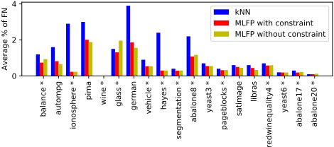
In the theoretical part of this paper, we have proved that learning a matrix M under the constraint λmax(M) ≤ 1 allows our algorithm to focus first on reducing FN. An illustration of the impact of this contraint in terms of false negatives is shown in Figure 4 on the 19 datasets. This figure reports the percentage of false negatives at test time generated by the 3NN algorithm and MLFP with or without the constraint. The results show that, compared to a 3NN algorithm, MLFP systematically reduces the number of false negatives and thus has the desired effect. When comparing MLFP with and without the constraint, we can note that on 14 datasets out of 19, the use of the constraint λmax(M) ≤ 1 leads at test time to a smaller number of false negatives.
6 Conclusion
In this paper, we have proposed a new metric learning algorithm to deal with imbalanced datasets. In this setting, finding the good compromise between the false negative and false positive rates is still an open problem. The original contribution of this paper comes from the optimization in our algorithm MLFP of a Mahalanobis distance which is only used to compare a new query to positive examples, while the Euclidean distance is still used when for comparing that query to negative samples. A constraint on the maximum eigenvalue of the learned matrix is introduced and has been shown to be provably efficient to reduce the false negative rate. Our paper is supported by a theoretical study and an extensive experimental evaluation showing that MLFP outperforms state-ofthe-art metric-learning methods.
This work opens the door to two promising lines of research. First, in MLFP we learn a linear projection of the data. One interesting perspective would consist in kernelizing our metric learning algorithm or designing a deep learning version allowing us to capture non linearity. A simpler solution might also consist in learning different local metrics for different regions of the input space as done in [Zantedeschi et al., 2016]. Second, as initiated in [Sharma et al., 2018], combining a Mahalanobis distance with a sampling strategy might lead to a new family of imbalanced learning methods.
Acknowledgements
This work was supported by the following projects: AURA project TADALoT (Pack Ambition 2017, 17 011047 01), ANR project LIVES (ANR-15-CE23-0026) and IDEXLYON project ACADEMICS (ANR-16-IDEX-0005).
@inproceedings{ijcai2020p298,
  title     = {Learning from Few Positives: a Provably Accurate Metric Learning Algorithm to Deal with Imbalanced Data},
  author    = {Viola, Rémi and Emonet, Rémi and Habrard, Amaury and Metzler, Guillaume and Sebban, Marc},
  booktitle = {Proceedings of the Twenty-Ninth International Joint Conference on
               Artificial Intelligence, {IJCAI-20}},
  publisher = {International Joint Conferences on Artificial Intelligence Organization},
  editor    = {Christian Bessiere},
  pages     = {2155--2161},
  year      = {2020},
  month     = {7},
  note      = {Main track},
  doi       = {10.24963/ijcai.2020/298},
  url       = {https://doi.org/10.24963/ijcai.2020/298},
}
TY - CPAPER TI - Learning from Few Positives: a Provably Accurate Metric Learning Algorithm to Deal with Imbalanced Data AU - Viola, Rémi AU - Emonet, Rémi AU - Habrard, Amaury AU - Metzler, Guillaume AU - Sebban, Marc T2 - Proceedings of the Twenty-Ninth International Joint Conference on Artificial Intelligence, IJCAI-20 PB - International Joint Conferences on Artificial Intelligence Organization PY - 2020 SP - 2155 EP - 2161 DO - 10.24963/ijcai.2020/298 UR - https://doi.org/10.24963/ijcai.2020/298 ER -Copied
Machine-readable versions of this paper, for tools and AI agents:





