Marthe: Scheduling the Learning Rate Via Online Hypergradients

1 Introduction

Learning rate (LR) adaptation for first-order optimization methods is one of the most widely studied aspects in optimization for learning methods, in particular neural networks. Recent research in this area has focused on developing complex schedules that depend on a small number of hyperparameters [Loshchilov and Hutter, 2017; Orabona and P´al, 2016] or proposed methods to optimize LR schedules w.r.t. the training objective [Schaul et al., 2013; Baydin et al., 2018; Wu et al., 2018]. While quick optimization is desirable, the true goal of supervised learning is to minimize the generalization error, which is commonly estimated by holding out part of the available data for validation. Hyperparameter optimization (HPO), a related but distinct branch of the literature, specifically focuses on this aspect, with less emphasis on the goal of rapid convergence on a single task. Research in this direction is vast and includes model-based, model-free, and gradient-based approaches (see [Hutter et al., 2019] for an overview). Additionally, works in the area of learning to optimize [Andrychowicz et al., 2016; Wichrowska et al., 2017] have focused on the problem of tuning parameterized optimizers on whole classes of learning problems but require prior expensive optimization and are not designed to speed up training on a single task.

∗Contact Author, Equal Contribution.

†Contact Author, Equal Contribution.

The goal of this paper is to automatically compute in an online fashion a learning rate schedule for stochastic optimization methods (such as SGD) only on the basis of the given learning task, aiming at producing models with associated small validation error. We study the problem of finding a LR schedule under the framework of gradient-based hyperparameter optimization [Franceschi et al., 2017]: we consider an optimal schedule η∗ = (η∗ 0 , . . . , η∗T-1 ) ∈ RT+ as a solution to the following constrained optimization problem

for t = {0, . . . , T - 1} = [T], where E : Rd → R+ is an objective function, Φt : Rd × R+ → Rd is a (possibly stochastic) weight update dynamics, ¯w ∈ Rd represents the initial model weights (parameters) and finally wt are the weights after t iterations. We can think of E as either the training or the validation loss of the model, while the dynamics Φ describe the update rule (such as SGD, SGDMomentum, Adam etc.). For example in the case of SGD, Φt(wt, ηt) = wt - ηt∇Lt(wt), with Lt(wt) the training loss on the t-th minibatch. The horizon T should be large enough so that the training error can be effectively minimized to avoid underfitting. A too large value of T does not necessarily harm since ηk = 0 for k > ¯ T is still a feasible solution, implementing early stopping in this setting. There is vast empirical evidence that the LR is among the most critical hyperparameters affecting the performances of learnt statistical models. Beside convergence arguments from the stochastic optimization literature, for all but the simplest problems, non-constant schedules yield generally better results [Bengio, 2012].

Problem (1) can be in principle solved by any HPO technique. However, most HPO techniques, including those based on hypergradients [Maclaurin et al., 2015] or on a bilevel programming formulation [Franceschi et al., 2018; MacKay et al., 2019] would not be suitable for the present purpose since they require multiple evaluations of f (which, in turn, require executions of the weight optimization routine). This clearly defeats one of the main goals of determining LR schedules, i.e. speed. In fact, several other researchers [Almeida et al., 1999; Schraudolph, 1999; Schaul et al., 2013; Franceschi et al., 2017; Baydin et al., 2018; Wu et al., 2018] have investigated related solutions for deriving greedy update rules for the learning rate. A common characteristic of methods in this family is that the LR update rule does not take into account information from the future. At a high level, we argue that any method should attempt to produce updates that approximate the true and computationally unaffordable hypergradient of the final objective with respect to the current learning rate. In relation to this, [Wu et al., 2018] discuss the bias deriving from greedy or short-horizon optimization. In practice, different methods resort to different approximations or explicitly consider greedily minimizing the performance after a single parameter update [Almeida et al., 1999; Schaul et al., 2013; Baydin et al., 2018]. The type of approximation and the type of objective (i.e. the training or the validation loss) are in principle separate issues although comparative experiments with both objectives and the same approximation are never reported in the literature. The validation loss is only used in experiments reported by Franceschi et al. [2017].

In this work, we make a step forward in understanding the behavior of online gradient-based hyperparameter optimization techniques by (i) analyzing in Section 2 the structure of the true hypergradient that could be used to solve Problem (1) if wall-clock time was not a concern, and (ii) by studying in Section 3 some failure modes of previously proposed methods along with a detailed discussion of the type of approximations that these methods exploit. In Section 4, based on these considerations, we develop a new hypergradient-based algorithm which reliably produces competitive learning rate schedules aimed at lowering the final validation error. The algorithm, which we call MARTHE (Moving Average RealTime Hyperparameter Estimation), has a moderate computational cost and can be interpreted as a generalization of the algorithms described by Baydin et al. [2018] and Franceschi et al. [2017]. In Section 5, we empirically compare the quality of different hypergradient approximations in a small scale task where true hypergradient can be exactly computed. In Section 6, we present a set of real world experiments showing the validity of our approach. We finally discuss potential future applications and research directions in Section 7.

2 Structure of the Hypergradient

We study the optimization problem (1) under the perspective of gradient-based hyperparameter optimization, where the learning rate schedule η = (η0, . . . , ηT-1) is treated as a vector of hyperparameters and T is a fixed horizon. Since the learning rates are positive real-valued variables, assuming both E and Φ are smooth functions, we can compute the gradient of f ∈ RT , which is given by

where "ᵀ" means transpose. The total derivative ˙wT can be computed iteratively with forward-mode algorithmic differentiation [Griewank and Walther, 2008; Franceschi et al., 2017] as

The Jacobian matrices At and Bt depend on wt and ηt, but we will leave these dependencies implicit to ease our notation. In the case of SGD 1 , At = I - ηtHt(wt) and [Bt]j = -δtj∇Lt(wt)ᵀ , where subscripts denote columns (starting from 0), δtj = 1 if t = j and 0 otherwise and Ht is the Hessian of the training error on the t-th mini-batch.

Given the high dimensionality of η, reverse-mode differentiation would result in a more efficient (running-time) implementation. We use here forward-mode both because it is easier to interpret and because it is closely related to the computational scheme behind MARTHE, as we will show in Section 4. We note that stochastic approximations of Eq. (2) may be obtained with randomized telescoping sums [Beatson and Adams, 2019] or hyper-networks based stochastic approximations [MacKay et al., 2019].

Eq. (3) describes the so-called tangent system [Griewank and Walther, 2008] which is a discrete affine time-variant dynamical system that measures how the parameters of the model would change for infinitesimal variations of the learning rate schedule, after t iterations of the optimization dynamics. Notice that the "translation matrices" Bt are very sparse, having, at any iteration, only one non-zero column. This means that [ ˙wt]j remains 0 for all j ≥ t: ηt affects only the future parameters trajectory. Finally, for a single learning rate ηt, the derivative (a scalar) is

where the last equality holds true for SGD. Eq. (5) can be read as the scalar product between the gradients of the training error at the t-th step and the objective E at the final iterate, transformed by the accumulated (transposed) Jacobians of the optimization dynamics, shorthanded by P T-1 t+1 in (6). As it is apparent from Eq. (5), given wt, the hypergradient of ηt is affected only by the future trajectory and does not depend explicitly on ηt.

In its original form, where each learning rate is left free to take any permitted value, Problem (1) presents a highly nonlinear setup. Although in principle it could be tackled by a projected gradient descent method, in practice this is not feasible even for relatively small problems: evaluating the gradient with forward-mode is inefficient in time since it requires maintaining a large matrix tangent system. Evaluating it with reverse-mode is inefficient in memory since the entire weight trajectory (wi)Ti=0 should be stored 2 . Furthermore, it can be expected that several updates of η are necessary to reach convergence - each update requiring the computation of fT and the entire parameter trajectory in the weight space. Since this approach is computationally very expensive, we turn out attention to online updates where ηt is required to be updated online based only on trajectory information up to time t.

1 Throughout we use SGD to simplify the discussion, however, similar arguments hold for any smooth optimization dynamics such as those including momentum terms.

2 Techniques based on implicit differentiation [Pedregosa, 2016; Agarwal et al., 2017] or fixed-point equations [Griewank and Faure, 2002] (also known as recurrent backpropagation [Pineda, 1988]) cannot be readily applied to compute ∇fT since the training loss L does not depend explicitly on η.

3 Online Gradient-Based Adaptive Schedules

Before developing and motivating our proposed technique, we discuss two previous methods to compute the learning rate schedule online. The real-time hyperparameter optimization (RTHO) algorithm suggested in [Franceschi et al., 2017], reminiscent of stochastic meta-descent [Schraudolph, 1999], is based on forward-mode differentiation and uses information from the entire weight trajectory by accumulating partial hypergradients. Hypergradient descent (HD), proposed in [Baydin et al., 2018] and closely related to the earlier work by Almeida et al. [1999], aims at minimizing the loss with respect to the learning rate after one step of optimization. It uses information only from the past and current iterate.

Both methods implement an update rules of the type

where ∆ηt is an online estimate of the hypergradient, β > 0 is a step-size or hyper-learning rate and the max ensures positivity 3 . To ease the discussion, we omit the stochastic (mini-batch) evaluation of the training error L and possibly of the objective E.

The update rules 4 are given by

for RTHO and HD respectively, where P t-1 t := I. Thus ∆RTHO = ∆HD + r((wi, ηi)t-2 i=0 ): the correction term r can be interpreted as an "on-trajectory approximations" of longer horizon objectives as we will discuss in Section 4.

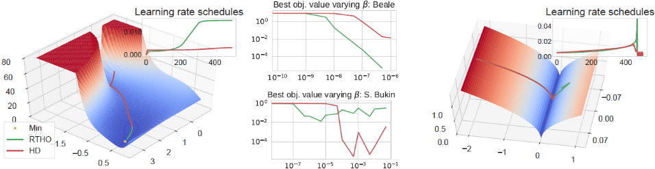
Although successful in some learning scenarios, we argue that both these update rules suffer from (different) pathological behaviors, as HD may be "shortsighted", being prone to underestimate the learning rate (as noted by Wu et al. [2018]), while RTHO may be too slow to adapt to sudden changes of the loss surface or, worse, it may be unstable, with updates growing uncontrollably in magnitude. We exemplify these behaviors in Figure 1, using two bidimensional test functions 5 from the optimization literature, where we set E = L and we perform 500 steps of gradient descent. The Beale function, on the left, presents sharp peaks and large plateaus. RTHO consistently outperforms HD for all probed values of β that do not lead to divergence (Figure 1 upper center). This can be easily explained by the fact that in flat regions gradients are small in magnitude, leading to ∆HDηt to be small as well. RTHO, on the other hand, by accumulating all available partial hypergradients and exploiting second order information, is capable of making faster progress. We use a simplified and smoothed version of the Bukin function N.6 to show the opposite scenario (Figure 1 lower center and right). Once the optimization trajectory closes the valley of minimizers y = 0.01x, RTHO fails to discount outdated information, bringing the learning rate first to grow exponentially, and then to suddenly vanish to 0, as the gradient changes direction. HD, on the other hand, correctly damps η and is able to maintain the trajectory close to the valley.

3 Updates could be also considered in the logarithmic space, e.g. by Schraudolph [1999]; we find it useful, to let η reach 0 whenever needed, offering a natural way to implement early stopping.

4 In [Franceschi et al., 2017], the hyperparameter is updated every K iterations. Here we focus on the case K = 1 which better allows for a unifying treatment. HD is developed using as objective the training loss L rather than the validation loss E. We consider here without loss of generality the case of optimizing E.

5 We use the Beale function defined as L(x, y) = (1.5 - x + xy)2 + (2.25 - x + xy2 )2 + (2.625 - x + xy3 )2 and a simplified smoothed version of Buking N.6: L(x, y) = √((y - 0.01x)2 + ε)1/2 + ε, with ε > 0.

These considerations suggest that neither ∆RTHO nor ∆HD provide globally useful update directions, as large plateaus and sudden changes on the loss surface are common features of the optimization landscape of neural networks [Bengio et al., 1994; Glorot and Bengio, 2010]. Our proposed algorithm smoothly interpolates between these two methods, as we will present next.

4 MARTHE

In this section, we develop and motivate MARTHE, an algorithm for computing LR schedules online during a single training run. This method maintains a moving-average over approximations of (5) of increasingly longer horizon, using the past trajectory and gradients to retain a low computational overhead. Further, we show that RTHO [Franceschi et al., 2017] and HD [Baydin et al., 2018] outlined above, can be interpreted as special cases of MARTHE, shedding further light on their behaviour and shortcomings.

Shorter horizon auxiliary objectives. For K > 0, define gK(u, ξ), with ξ ∈ RK+ as

The gKs define a class of shorter horizon objective functions, indexed by K, which correspond to the evaluation of E after K steps of optimization, starting from u ∈ Rd and using ξ as the LR schedule 6 . Now, the derivative of gK with respect to ξ0, denoted g′K , is given by

where the last equality holds for SGD dynamics. Once computed on subsets of the original optimization dynamics (wi)Ti=0 , the derivative reduces for K = 1 to g′1 (wt, ηt) = -∇E(wt+1)∇L(wt)ᵀ (for SGD dynamics), and for K = T - t to g′T-t (wt, (ηi)T-1 i=t ) = [∇f(η)]t . Intermediate values of K yield cheaper, shorter horizon approximations of (5).

6 Formally, ξ and u are different from η and w from the previous sections; later, however, we will evaluate the gK's on subsequences of the optimization trajectory.

Algorithm 1 MARTHE; requires β, µ, η0[= 0]

Initialization of w and Z0 ← 0

for t = 0 to T do

end for

Algorithm 1 presents the pseudocode of MARTHE. The runtime and memory requirements of the algorithm are dominated by the computation of the variables Z. Being these structurally identical to the tangent propagation of forward mode algorithmic differentiation, we conclude that the runtime complexity is only a multiplicative factor higher than that of the underlying optimization dynamics Φ and requires two times the memory (see Griewank and Walther [2008], Sec. 4).

5 Optimized Schedules and Quality of MARTHE Approximations

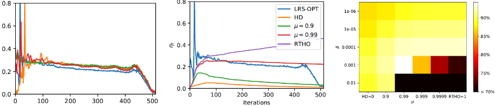
In this section, we empirically compare the optimized LR schedules found by approximately solving Problem 1 by gradient descent (denoted LRS-OPT), where the hypergradient is given by Eq. (5), against those generated by MARTHE, for a wide range of hyper-momentum factors µ (including HD and RTHO) and hyper-learning rates β. We are interested in understanding and visualizing the qualitative similarities among the schedules, as well as the effect of µ and β on the final performance measure. To this end, we trained threelayers feed forward neural networks with 500 hidden units per layer on a subset of 7000 MNIST [LeCun et al., 1998] images. We used a cross-entropy loss and SGD as optimization dynamics Φ, with a mini-batch size of 100. We further sampled 700 images to form the validation set and defined E to be the validation loss after T = 512 optimization steps (about 7 epochs). For LRS-OPT, we randomly generated different mini-batches at each iteration, to prevent the schedule from unnaturally adapting to a specific progression of minibatches 7 . We initialized η = 0.01 · 1512 for LRS-OPT and set

7 We retained, however, the random initialization of the network weights, to account for the impact that this may have on the initial part of the trajectory. This offers a fairer comparison between LRSOPT and online methods, which compute the trajectory only once.

Approximating the future trajectory with the past. Explicitly using any of the approximations given by g′K (wt, η) as ∆ηt is, however, still largely impractical, especially for K ≫ 1. Indeed, it would be necessary to iterate the map Φ for K steps in the future, with the resulting (wt+i)Ki=1 iterations discarded after a single update of the learning rate. For K ∈ [t], we may then consider evaluating g′K exactly K steps in the past, that is evaluating g′K (wt-K, (ηi)t-1 i=t-K ). Selecting K = 1 is indeed equivalent to ∆HD, which is computationally inexpensive. However, when past iterates are close to future ones (such as in the case of large plateaus), using larger K's would allow in principle to capture longer horizon dependencies present in the hypergradient structure of Eq. (5). Unfortunately the computational efficiency of K = 1 does not generalize to K > 1, since setting ∆ηt = g′K would require maintaining K different tangent systems.

Discounted accumulation of g′k s. The definition of the gKs, however, allows one to highlight the recursive nature of the accumulation of g′K . Indeed, by maintaining the vector tangent system,

with Zi ∈ Rd , computing the moving average

from SK-1 requires only updating (14) and recomputing the gradient of E. The total cost of this operation is O(c(Φ)) per step both in time and memory using fast Jacobians vector products [Pearlmutter, 1994] where c(Φ) is the cost of computing the optimization dynamics (typically c(Φ) = O(d)). The parameter µ ∈ [0, 1] allows to control how quickly past history is forgotten. One can notice that ∆RTHOηt = St,1(w0, (ηj )t-1 i=0 ), while µ = 0 recovers ∆HDηt. Values of µ < 1 help discounting outdated information, while as µ increases so does the horizon of the hypergradient approximations. The computational scheme of Eq. (14) is quite similar to that of forward-mode algorithmic differentiation for computing ˙w (see Section 2 and Eq. (3)); however, the "tangent system" in Eq. (14), exploiting the sparsity of the matrices Bt, only keeps track of the variations with respect to the first component ξ0, drastically reducing the running time.

η0 = 0.01 for MARTHE, and repeated the experiments for 4 random seeds.

Figure 2 (left) shows the LRS-OPT schedules found after 5000 iterations of gradient descent: the plot reveals a strong initialization (random seed) specific behavior of η∗ for approximately the first 100 steps. The LR schedule then stabilizes or slowly decreases up until around 50 iterations before the final time, at which point it quickly decreases (recall that, in this setting, all ηi, including η0, are optimized "independently" and may take any permitted value). Figure 2 (center) present a qualitative comparison between the offline LRS-OPT schedule and the online ones, for indicative values of µ. Too small values of µ result in an underestimation of the learning rates, with generated schedules that quickly decay to very small values - this is in line with what observed in [Wu et al., 2018]. For too high values of µ (µ = 1 i.e. RTHO [Franceschi et al., 2017] in the figure) the schedules linger or fail to decrease, possibly causing instability and divergence. For certain values of µ, the schedules computed by MARTHE seems to capture the general behaviour of the optimized ones. Finally, Figure 2 (right) shows the average validation accuracy (rather than loss, for easier interpretation) of MARTHE methods varying β and µ. Higher values of µ translate to higher final performances - with a clear jump occurring between µ = 0.9 and µ = 0.99 - but may require a smaller hyper learning rate to prevent divergence.

6 Experiments

We performed an extensive set of experiments in order to compare MARTHE, RTHO, and HD. We also considered a classic LR scheduling baseline in the form of exponential decay (Exponential) where the LR schedule is defined by ηt = η0γ t . The purpose of these experiments is to perform a thorough comparison of various learning-rate scheduling methods, with a focus on those that are (hyper-)gradient based, in the fairest possible manner: indeed, these methods have very different running-time per iteration - HD and Exponential being much faster than MARTHE and RTHO - as well as different configuration spaces. It would be unfair to compare them using the number of iterations as computational budget. We therefore designed an experimental setup that allowed us to account for it: we implemented a random search strategy over the respective algorithms' configuration spaces and early-stopped each run with a 10-epochs patience window. We repeatedly drew configurations parameters (hyperhyperparameters) and run respective experiments until a fixed time budget of 36 hours was reached. The proposed experimental setting tries to mimic how machine learning practitioners may approach the parameter-tuning problem.

We used two alternative optimization dynamics: SGDM with the momentum hyperparameter fixed to 0.9 and Adam with the commonly suggested default values β1 = 0.9 and β2 = 0.999. We fixed the batch size to 128, the initial learning rate η0 = 0.1 for SGDM and 0.003 for Adam, and the weight decay (i.e. 2-norm) to 5·10-4 . For the adaptive methods, we sampled β in [10-3 , 10-6 ] log-uniformly, and for our method, we sampled µ between 0.9 and 0.999. Finally, we picked the decay factor γ for Exponential log-uniformly in [0.9, 1.0].

In our first set of experiments, we used VGG-11 [Simonyan and Zisserman, 2014] with batch normalization [Ioffe and Szegedy, 2015] after the convolutional layers, on CIFAR10 [Krizhevsky and Hinton, 2009], and SGDM as the inner optimizer. In the second set of experiments, we used ResNet-18 [He et al., 2016] on CIFAR100 [Krizhevsky and Hinton, 2009], in this case with Adam. For both CIFAR10 and CIFAR100, we used 45000 images as training images and 5000 images as the validation dataset. An additional set of 10000 test images was finally used to estimate generalization accuracy. We used standard data augmentation, including mean-std normalization, random crops and horizontal flips. Gradients were clipped to an absolute value of 100.0.

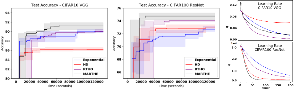
We kept track of the model with the best validation accuracy found so far, reporting in Figure 3 (left and center) the relative mean test accuracy (solid line) and minimum and maximum (limits of the shaded regions) across 5 repetitions. Inspecting the figure, it is possible to identify which method is the best performing one for any give time budget, both in average and in the worst/best case scenario. Figures 3 (right) shows examples of the LR schedules obtained by using the different methods.

We performed all experiments using AWS P3.2XL instances, each providing one NVIDIA Tesla V100 GPU. Finally, our PyTorch implementation of the methods and the experimental framework to reproduce the results is available at https://github.com/awslabs/adatune.

6.1 Discussion

In the analysis of our results, we will mainly focus on the accuracy on the test dataset achieved by different methods within a fixed time budget. For all the experiments, results summarized in Figure 3 show that both Exponential and HD were able to obtain a reasonably good accuracy within the first 4 hours, while RTHO and MARTHE required 6 hours at least to reach the same level of accuracy. This is due to the fact that the wall-clock time required to process a single minibatch is different: MARTHE takes approximately 4 times the wall-clock time of HD; there is negligible wallclock time difference between MARTHE and RTHO or between HD and Exponential. MARTHE was able to surpass all the other methods consistently after 10 hours.

Our experimental protocol resulted in HD and Exponential getting more trials compared to RTHO and MARTHE (in average around 24 trials for the first two compared to 8 of RTHO and MARTHE). Despite the fact that MARTHE could only afford fewer trials, it could still achieve better performance, suggesting that it is able to produce better learning rate schedules more reliably. Moreover, MARTHE maintains a better peak accuracy compared to RTHO showing the effectiveness of down-weighting outdated information.

Our experimental setup helped us investigate the robustness of the methods with respect to the choice of the hyperhyperparameters 8 . To that end, we can see from Figure 3 (left) that the average and worst case test set accuracies (measured across multiple seeds) of MARTHE are better in comparison to the other methods. This is a strong indication that MARTHE demonstrated superior adaptability with respect to different hyper-hyperparameters and seeds compared to other methods. This is also reflected by the result that MARTHE outperforms other strategies on a consistent basis if given a sufficient time budget (4-6 hours in our experiments): the higher computational cost of MARTHE is outbalanced by the fact that it needs fewer trials to reach the same performance level of faster methods like Exponential or HD.

8 We note that it is not common in the existing literature to mention the necessity of tuning hyper-hyperparameters for adaptive learning-rate methods, although different datasets and/or networks may require some tuning that may strongly affect the results.

Overall, our experiments reveal that RTHO and MARTHE provide better performance, giving a clear indication of the importance of the past information. Due to its lower computational overhead, Exponential should be still preferred under tight budget constraints, while MARTHE with µ ∈ [0.9, 0.999] should be preferred if enough time is available.

7 Conclusion

Finding a good learning rate schedule is an old but crucially important issue in machine learning. This paper makes a step forward, analyzing previously proposed online gradientbased methods and introducing a more general technique to obtain performing LR schedules based on an increasingly long moving average over hypergradient approximations. MARTHE interpolates between HD and RTHO, and its implementation is fairly simple within modern automatic differentiation, adding only a moderate computational overhead over the underlying optimizer complexity.

In this work, we studied the case of optimizing the learning rate schedules for image classification tasks; we note, however, that MARTHE is a general technique for finding online hyperparameter schedules (albeit it scales linearly with the number of hyperparameters), possibly implementing a competitive alternative in other application scenarios, such as tuning regularization parameters [Luketina et al., 2016]. We plan to further validate the method both in other learning domains for adapting the LR and also to automatically tune other crucial hyperparameters. We believe that another interesting future research direction could be to derive or learn adaptive rules for µ and β.