
Multi-Channel Graph Neural Networks
Proceedings of the Twenty-Ninth International Joint Conference on Artificial Intelligence. Main track. Pages 1352-1358.
https://doi.org/10.24963/ijcai.2020/188
Keywords
- Data Mining: Mining Graphs, Semi Structured Data, Complex Data
- Data Mining: Applications
- Data Mining: Classification, Semi-Supervised Learning
Abstract
The classification of graph-structured data has be-come increasingly crucial in many disciplines. It has been observed that the implicit or explicit hierarchical community structures preserved in real-world graphs could be useful for downstream classification applications. A straightforward way to leverage the hierarchical structure is to make use the pooling algorithms to cluster nodes into fixed groups, and shrink the input graph layer by layer to learn the pooled graphs.However, the pool shrinking discards the graph details to make it hard to distinguish two non-isomorphic graphs, and the fixed clustering ignores the inherent multiple characteristics of nodes. To compensate the shrinking loss and learn the various nodes’ characteristics, we propose the multi-channel graph neural networks (MuchGNN). Motivated by the underlying mechanisms developed in convolutional neural networks, we define the tailored graph convolutions to learn a series of graph channels at each layer, and shrink the graphs hierarchically to en-code the pooled structures. Experimental results on real-world datasets demonstrate the superiority of MuchGNN over the state-of-the-art methods.
- [Abu-El-Haija et al., 2018] Sami Abu-El-Haija, Amol Kapoor, Bryan Perozzi, and Joonseok Lee. N-gcn: Multi-scale graph convolution for semi-supervised node classification. arXiv preprint arXiv:1802.08888, 2018.
- [Aditya and Jure, 2016] Grover Aditya and Leskovec Jure. node2vec: Scalable feature learning for networks. In Pro- ceedings of the 22nd ACM SIGKDD international con- ference on Knowledge discovery and data mining, pages 855-864, 2016.
- [Aynaz Taheri, 2018] Tanya Berger-Wolf Aynaz Taheri, Kevin Gimpel. Learning graph representations with recurrent neural network autoencoders. In KDD'18 Deep Learning Day, 2018.
- [Borgwardt et al., 2005] Karsten M Borgwardt, Cheng Soon Ong, Stefan Schönauer, SVN Vishwanathan, Alex J Smola, and Hans-Peter Kriegel. Protein function predic- tion via graph kernels. Bioinformatics, 21(suppl 1):i47- i56, 2005.
- [Bruna et al., 2013] Joan Bruna, Wojciech Zaremba, Arthur Szlam, and Yann LeCun. Spectral networks and lo- cally connected networks on graphs. arXiv preprint arXiv:1312.6203, 2013.
- [D Dobson and Doig, 2003] Paul D Dobson and Andrew Doig. Distinguishing enzyme structures from non- enzymes without alignments. Journal of molecular biol- ogy, 330:771-83, 08 2003.
- [Dai et al., 2016] Hanjun Dai, Bo Dai, and Le Song. Dis- criminative embeddings of latent variable models for structured data. In ICML, pages 2702-2711, 2016.
- [Duvenaud et al., 2015] David K Duvenaud, Dougal Maclaurin, Jorge Iparraguirre, Rafael Bombarell, Tim- othy Hirzel, Alán Aspuru-Guzik, and Ryan P Adams. Convolutional networks on graphs for learning molecular fingerprints. In Advances in neural information processing systems, pages 2224-2232, 2015.
- [Gao and Ji, 2019] Hongyang Gao and Shuiwang Ji. Graph u-net, 2019.
- [Geng et al., 2019] Xu Geng, Yaguang Li, Leye Wang, Lingyu Zhang, Qiang Yang, Jieping Ye, and Yan Liu. Spatiotemporal multi-graph convolution network for ride- hailing demand forecasting. In 2019 AAAI Conference on Artificial Intelligence (AAAI'19), 2019.
- [Hamilton et al., 2017] Will Hamilton, Zhitao Ying, and Jure Leskovec. Inductive representation learning on large graphs. In Advances in Neural Information Processing Systems, pages 1024-1034, 2017.
- [Ioffe and Szegedy, 2015] Sergey Ioffe and Christian Szegedy. Batch normalization: Accelerating deep network training by reducing internal covariate shift. International Conference on Machine Learning, 2015.
- [Kipf and Welling, 2017] Thomas N Kipf and Max Welling. Semi-supervised classification with graph convolutional networks. ICLR, 2017. [Krizhevsky et al., 2012] Alex Krizhevsky, Ilya Sutskever, and Geoffrey E Hinton. Imagenet classification with deep convolutional neural networks. In Advances in neural in- formation processing systems, pages 1097-1105, 2012.
- [Niepert et al., 2016] Mathias Niepert, Mohamed Ahmed, and Konstantin Kutzkov. Learning convolutional neural networks for graphs. In International conference on ma- chine learning, pages 2014-2023, 2016.
- [Shervashidze et al., 2011] Nino Shervashidze, Pascal Schweitzer, Erik Jan van Leeuwen, Kurt Mehlhorn, and Karsten M Borgwardt. Weisfeiler-lehman graph kernels. Journal of Machine Learning Research, 12(Sep):2539- 2561, 2011.
- [Simonovsky and Komodakis, 2017] Martin Simonovsky and Nikos Komodakis. Dynamic edge-conditioned filters in convolutional neural networks on graphs. In Proceedings of the IEEE conference on computer vision and pattern recognition, pages 3693-3702, 2017.
- [Vaswani et al., 2017] Ashish Vaswani, Noam Shazeer, Niki Parmar, Jakob Uszkoreit, Llion Jones, Aidan N Gomez, Łukasz Kaiser, and Illia Polosukhin. Attention is all you need. In Advances in Neural Information Processing Sys- tems, pages 5998-6008, 2017.
- [Velickovic et al., 2017] Petar Velickovic, Guillem Cucurull, Arantxa Casanova, Adriana Romero, Pietro Lio, and Yoshua Bengio. Graph attention networks. arXiv preprint arXiv:1710.10903, 1(2), 2017.
- [Xu et al., 2018] Keyulu Xu, Weihua Hu, Jure Leskovec, and Stefanie Jegelka. How powerful are graph neural net- works? arXiv preprint arXiv:1810.00826, 2018.
- [Yanardag and Vishwanathan, 2015] Pinar Yanardag and S. V. N. Vishwanathan. A structural smoothing framework for robust graph comparison. In Advances in Neural Information Processing Systems, 2015.
- [Ying et al., 2018] Zhitao Ying, Jiaxuan You, Christopher Morris, Xiang Ren, Will Hamilton, and Jure Leskovec. Hierarchical graph representation learning with differen- tiable pooling. In NeurIPS, pages 4805-4815, 2018.
- [Zhang et al., 2018a] Muhan Zhang, Zhicheng Cui, Marion Neumann, and Yixin Chen. An end-to-end deep learning architecture for graph classification. In Association for the Advancement of Artificial Intelligence, 2018.
- [Zhang et al., 2018b] Xi Zhang, Lifang He, Kun Chen, Yuan Luo, Jiayu Zhou, and Fei Wang. Multi-view graph convo- lutional network and its applications on neuroimage anal- ysis for parkinson's disease. In AMIA Annual Symposium Proceedings, volume 2018, page 1147. American Medical Informatics Association, 2018.
- [Zhou et al., 2019] Kaixiong Zhou, Qingquan Song, Xiao Huang, and Xia Hu. Auto-gnn: Neural architec- ture search of graph neural networks. arXiv preprint arXiv:1909.03184, 2019.
References were extracted automatically from the PDF and may contain errors.
Full text extracted automatically from the PDF; figures, tables and equations may differ. The PDF is the version of record.
1 Introduction
Classifying the graph-structured data has become an important problem in various domains, such as the biological graph and chemical molecule analysis [Aynaz Taheri, 2018]. In predicting the associated label of a graph structure, one of the most effective information is the pooled structures present inherently in real-world graph. For example, the pooled structures defined by the nodes' communities and their correlation determines the outline relationship in social media [Aditya and Jure, 2016]. The local molecular structures would significantly influence the properties of a molecule.
To take advantage of the implicit or explicit pooled structures, a straightforward way is to shrink and learn the input graph hierarchically [Ying et al., 2018; Gao and Ji, 2019]. The hierarchical graph neural networks (GNN) are set up based on two main components: pooling algorithm and GNN. The pooling algorithm is used to cluster nodes of the input graph and then formulate pooled graphs layer by layer. It is comparable with the pooling layer in convolutional neural networks (CNN) [Krizhevsky et al., 2012], which coarsen image resolution to extract the hierarchically global knowledge. Given the pooled graph at each layer, GNN model is applied to learn embedding representations of the node communities [Bruna et al., 2013; Velickovic et al., 2017; Vaswani et al., 2017; Zhou et al., 2019]. The core idea is to update a node via aggregating the representations of itself and its neighbors to learn the neighborhood structure. To classify the input graph, its latent representation could be generated by summarizing all the representations of node communities at the last layer of hierarchical GNN [Shervashidze et al., 2011; Duvenaud et al., 2015; Dai et al., 2016].
However, the direct applications of hierarchical GNN are still problematic for classifying graphs because of the following two reasons. First, the pooling algorithm discards edge details to shrink the input graph. Given two non-isomorphic graphs, they may be pooled into the same ones at the higher layers, and possess the similar and indistinguishable graph representations. Second, the pooling algorithm only captures the partial characteristics of nodes, and clusters them fixedly to learn a single pooled structure at each layer. Generally, nodes in the real-world graphs could play various roles and belong to different communities simultaneously. In other words, they could be naturally clustered from multiple views to formulate the distinct pooled graphs. Thus, the single pooled graph in the existing work may fail to preserve the multiple nodes' characteristics.
To tackle the above problems, we propose the multichannel GNN framework which encodes a series of pooled graphs layer by layer. The graph series at each layer learns the various characteristics of nodes to compensate the graph shrinking, and improve the capability to distinguish the nonisomorphic graphs. Via clustering the nodes learned with various characteristics, the graph series keeps the multi-view pooled structures of the input graph. The proposed framework is motivated by CNN from the image domain, where both the convolutional filter and pooling layer work together to operate on image channels hierarchically. The grid-like image could be regarded as a special type of graph-structured data, at which the pixel is represented by a node. Each pixel has 8 directly adjacent pixels located from the upper left to the lower right. However, there are two challenges in building up such a deep neural network for the general graph-structured data. First, across each graph, the nodes have various numbers and uncertain orders of their neighbors. The local convolutions in CNN cannot be directly applied to learn the nodes' characteristics to formulate the graph series, since it is predefined with the shape of local neighbors. Several attempts [Abu-El-Haija et al., 2018; Geng et al., 2019; Zhang et al., 2018b] have been made to handle this challenge by manually predefining the adjacency matrix, which is not generalizable. Second, considering the pooled graph series as shown by (X1 ,A1 ) and (X2 ,A2 ) in Figure 1, they have the pooled structures with different physical meaning. The nodes of one channel cannot be mapped to those of the other, since they are clustered from the different patches. The edges also cannot be mapped because they connect the different node clusters. That prevents us from using the channel-wise convolutional filters in CNN to aggregate these graph series to generate the new pooled graphs at the next layer. The filters could only sum up the grid-like image channels with the same physical meaning in the pixels.
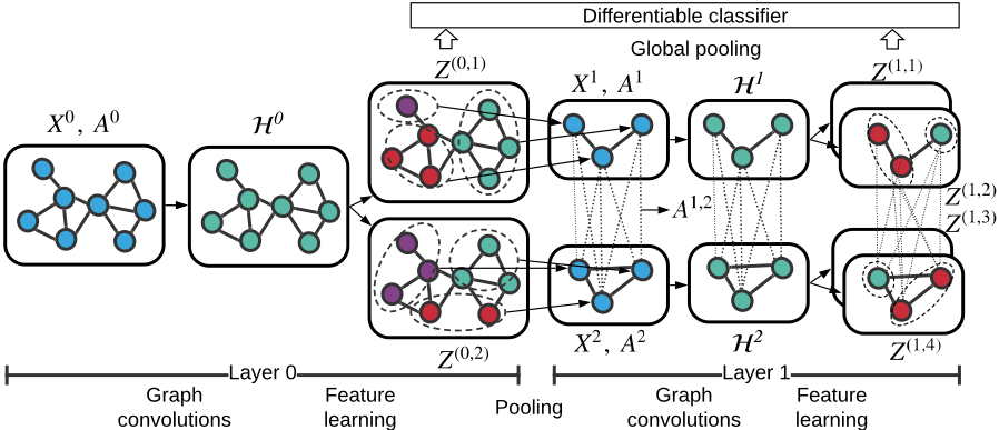
We address the above challenges by developing the multichannel graph neural networks (MuchGNN) as shown in Figure 1. To be specific, it could be separated as the following two research questions. (i) How to define the convolutional filters to learn the various nodes' characteristics to formulate the pooled graph series? (ii) How to define the graph convolutions to aggregate the distinct pooled graphs? In summary, our major contributions are described below.
- We propose a multi-channel GNN framework, at which a series of pooled graphs are encoded hierarchically.
- We design the convolutional filter to learn the node characteristics without reliance on the neighborhood shape.
- We define the inter-channel graph convolutions to aggregate the graph channels via message passing.
2 Preliminaries
The goal of graph classification is to map graphs into a set of labels. Let G = (A,X) denote the directed or undirected graph consisting of n nodes, where A ∈ {0, 1}n×n denotes the adjacency matrix, and X ∈ Rn×d denotes the feature matrix in which each row represents a d-dimensional feature vector of a node. Given a set of graphs {G1, . . . ,GN} ⊂ G and the corresponding labels {y1, . . . , yN} ⊂ Y, the challenge is to learn the graph representations to facilitate the following graph classification: f : G →Y.
2.1 Graph Neural Networks
GNN uses the adjacency structure and node features to learn the node embeddings. A general "message-passing" based GNN could be expressed by [Xu et al., 2018]:
where Hk denotes the hidden node embedding after k steps of graph convolutions, Wk ∈ Rd×d denotes the trainable transformation matrix, and σ denotes the ReLU activation function. We initialize H0 by input feature X. Node embedding is updated by aggregating the representations of its neighbors and itself. After K steps of message passing, we could reach out to the neighbors that are at maximumK hops away from the central node. For the ease of presentation, we denote GNN associated with K steps of message passing as Z = GNN(A,X) ∈ Rn×d . The representation of a graph is generated by aggregating the n node embeddings in matrix Z for classification purpose.
2.2 Differentiable Pooling
A major limitation of Equation (1) is that it only encodes the superficial structure of input graph. Recently, the differentiable pooling [Ying et al., 2018] (DIFFPOOL) is proposed to cluster nodes from the input graph gradually, and generates the pooled graphs layer by layer. Formally, let nl and nl+1 denote the node numbers of pooled graphs at layers l and l + 1, respectively. Generally we have nl+1 < nl < n in order to obtain the more abstract graphs at the higher layers of model. Let S(l) ∈ Rnl×nl+1 and Z (l) ∈ Rnl×d denote the cluster assignment matrix and node embedding learned at layer l, respectively. The DIFFPOOL module pools a graph from layer l to l + 1 as follows:
A(l+1) and X(l+1) denote the adjacency and node feature matrices of the graph at layer l + 1, respectively. To prepare the cluster matrix S(l) and node embedding Z (l) , two GNN modules are used: Z (l) = GNNl,embed(A(l) , X(l) ) and S(l) = softmax(GNNl,pool(A(l) ,X(l) )). The softmax function is applied in row-wise fashion to determine the probabilities of assigning each node at layer l to the clusters at layer l+1. Given the pooled graphs at all layers, GNNs are applied hierarchically to obtain their representations by aggregating the embeddings of the corresponding node clusters.
3 Multi-channel Graph Convolutional Networks
The pooling algorithm has its own bottlenecks in graph representation learning. The input graph is pooled and distorted gradually, which makes it hard to distinguish heterogeneous graphs at higher layers. The single pooled graph at each layer cannot preserve the inherent multi-view pooled structures. To tackle these issues, we propose MuchGNN to learn the graph-structured data comparable with CNN learning the image data. As shown in Figure 1, a series of convolutional filters is applied to study the various characteristics of nodes before pooling, and compensates the clustering distortion. Given the graphs learned with the series of convolutional filters, the pooling algorithm clusters nodes in different ways to encode the multi-view pooled structures at the next layer.
Compared with CNN, the challenges of building up MuchGNN lie in the following two facts. First, nodes across the graph have different numbers of direct neighbors. For example, the upper-left node in graph {X0 ,A0 } has only one neighbor as shown in Figure 1, while the others have at least two. There is also none related orders for all the neighbors of one node. The non-determined neighborhood shape precludes us from directly applying the filter in CNN to learn the nodes' characteristics, such as filter 3 × 3 × 128 pre-defining the neighborhood shape of heights, widths and channels. Second, such channel-wise convolutional filter cannot combine the pooled graphs at one layer together to aggregate their features, and then generate the new one at the next layer. That is because the nodes and edges of one pooled graph are hard to be mapped to those of the another. We cannot combine two pooled graphs in the node-wise and edge-wise fashions.
MuchGNN addresses the above challenges with two key components: (i) the convolutional filter defined based on the message passing steps in GNN, instead of the direct neighbors; (ii) the specific graph convolutions passing messages among the pooled graphs to aggregate their features. For the consistency of presentation, we first define two key concepts.
Definition 1: layer. A layer is composed of operations of graph convolutions and feature learning as shown in Figure 1. Let l denote the index of layer. The input to layer l is a set of graphs (e.g., [{X1 ,A1 }, {X2 ,A2 }] at layer 1), while the output is a series of graphs associated with the learned node embeddings (e.g., [Z (1,1) , · · · ,Z (1,4) ] at layer 1).
Definition 2: channel. Given a specific layer, a channel represents the input graph denoted by Gi = {Xi , Ai }, where i denotes the channel index. As shown in Figure 1, layer 0 consists of one channel: [G0 = {X0 ,A0 }], and layer 1 consists of two channels [G1 = {X1 , A1 }, G2 = {X2 , A2 }].
3.1 ProposedMethods
As shown in Figure 1, we first describe how MuchGNN learns the various nodes' characteristics in the single channel at layer 0 by defining the graph convolutional filters. Following this, we describe how MuchGNN operates the graph convolutions to pass message among the multiple channels at layer 1. Without loss of generality, we explain the main ideas of MuchGNN upon the structure of message-passing GNN and differentiable pooling. The proposed framework could be easily applied on other GNNs and pooling algorithms.
Single-channel Learning Process
Considering channel i = 0 at layer l = 0, graph G0 = {X0 , A0 } is initialized by the input graph G = {X, A}. The single-channel learning process includes two states: graph convolutions and feature learning. The graph convolutions stage applies GNN model to obtain node embeddings via K steps of message passing. Node embedding of the k-th step,
W (l) k denotes the trainable parameter for the k-th message passing for all channels at layer l. Based onWeisfeiler-Leman (WL) algorithm [Xu et al., 2018], the two non-isomorphic graphs could only be distinguished if their node embeddings Hik are different at any step k. To learn the nodes' characteristics informative for classifying graphs, we make use of multiset Hi = [Xi ,Hik ] that contains the input feature and all the intermediate node embeddings, where k = 1, · · · ,K. The feature learning stage then generates the series of new graphs, each of which is associated with a node embedding matrix learned from a corresponding trainable filter. Formally, filter θ(l,j) ∈ R1×(K+1) learns the new graph associated with embedding Z (l,j) as follows:
Index tuple (l, j) denotes the j-th newly generated graphs at layer l, and b is a trainable scalar. We have (l, j) = (0, 1) and (0, 2) at layer 0 as shown in Figure 1. φ, sum and ⊙ denote the non-linear function of multilayer perceptron (MLP), the summation function and the element-wise multiplication, respectively. Note that filter θ(l,j) learns the nodes' characteristic by taking into account the different steps of message passing, rather than relying on the direct neighbors of nodes. Following the same process of graph convolution and feature learning, we obtain cluster matrices S(l,j) for the two new graphs through another GNN model and convolutional filters.
Given embeddings Z (l,j) and S(l,j) at the j-th graph, the clustering algorithm defined in Equation (2) is applied to formulate channel j at the next layer. We have channels G1 = {X1 ,A1 } and G2 = {X2 ,A2 } at layer 1, which encode the diverse pooled structures of input graph.
Multi-channel Learning Process
Unlike layer 0, the input to layer 1 is given by a series of channels. The graph convolutions stage requires feature aggregation from this series of channels to generate the more abstract representation at the higher layer of model. Recalling the graph convolutions at layer 0, it is an intra-channel graph convolutions that pass message only within the current channel. In this section, we augment the graph convolutions by further defining an inter-channel graph convolutions to aggregate features from neighboring channels to the current one.
To unify the following expression, we denote the current and neighboring channels with indices i and c, respectively. Considering the graph convolutions operated on graph G1 = {X1 ,A1 } of current channel i = 1, it includes both intrachannel and inter-channel components to receive information from current channel i = 1 and neighboring channel c = 2, respectively. The intra-channel graph convolutions is given by Equation (3), where the indices of channel and layer are i = 1 and l = 1. Following the message-passing GNN, we define the inter-channel graph convolutions as follows:
Hi,c k denotes the node embedding of channel i, after k steps of feature aggregations from neighboring channel c. At step 0, embedding Hi,c 0 is given by Xi of current channel i. Ai,c denotes the inter-channel adjacency matrix between channels i and c, at which i = 1 and c = 2 at layer 1. Following the pooling algorithms in Equation (2), the inter-channel adjacency matrix is easy to obtain by: A1,2 = S(0,1)T A0S(0,2) ∈ Rn1×n1 . The row and column of A1,2 represent the nodes at channels 1 and 2, respectively. Compared with the intrachannel convolutions, we replace the adjacency matrix with Ai,c . In this way, the messages of neighboring channels c could be passed to update the embedding at channel i despite the different shapes of their graph structures.
Following the graph convolutions, the feature learning stage learns the nodes' characteristics based on Equation (4). Different frommultiset H0 in the single-channel scenario, the one at channel i is given by Hi = [Xi , Hik , Hi,c k ] at the higher layer of model. It includes embeddings Hi,c k to aggregate features from all the neighbor channels c. Specifically, we have H1 = [X1 ,H1 k , H1,2 k ] at channel 1. Given a set of filters θ(l,j) , Equation (4) encodes the various characteristics and obtains a series of graphs from channel 1. As shown in Figure 1, they are denoted by Z (1,1) and Z (1,2) , respectively. By repeating the previous process for channel 2, we obtain the graphs associated with embeddings Z (1,3) and Z (1,4) .
Multi-channel Graph Convolutional Networks
We stack L layers of graph convolutions and feature learning in MuchGNN, at which L = 2 in Figure 1. Let nl and Cl denote the node number of a graph and the channel number at layer l, respectively. We define rl ≜ nl+1 nl named assign ratio, and define Tl ≜ Cl+1 Cl named channel expansion. Generally, cluster algorithm requires 0 < rl ≤ 1 to generate pooled graph structures, and our feature learning applies Tl > 1 to learn the various characteristics of nodes. For each layer l, we generate a series of graphs whose node embeddings are Z (l,j) , j = 1, · · · ,ClTl. As shown in Figure 1, we have C1T1 = 2 × 2 at layer 1. The graph representation Y (l) learned at layer l is obtained by combining graphs as follows:
where GlobalPool denotes the global pooling function to read out the graph representation. The entire graph representation Y is generated by concatenating Y (l) from all the layers: Y = ⊕lY (l) ∈ Rd·L×1 . It encodes both the input graph and its multi-view pooled structures. Given the input of Y , the downstream differentiable classifier, like MLP, is applied to predict the corresponding graph label.
3.2 Complexity Analysis
Considering channel i at layer l, we analyze the time complexity to learn the node's characteristics based on Equation (4). First, node embeddings Hik and Hi,c k within multiset Hi need to be prepared according to Equations (3) and (5), respectively. Let m denote the maximum number of edges within channel i or between channels i and j. The complexities of Equations (3) and (5) are O(md2 ) and O(nld2 + md2 ), respectively. There are total K steps of message passing and Cl - 1 neighboring channels waited to be aggregated. Therefore, the time cost to obtain multiset Hi is O(K[Clmd2 + (Cl - 1)nld2 ]). Second, the element-wise multiplication in Equation (4) takes the computation cost of O((KCl + 1)nld). Based on the above two components, the total time complexity in feature learning is O(K[Clmd2 + (Cl - 1)nld2 ] + (KCl + 1)nld), which increases linearly with step K and channels Cl.
4 Experiments
We evaluate MuchGNN to answer the following questions:
- Q1: How does MuchGNN perform when it is compared with other state-of-the-art models?
- Q2: How does the multiple channels in MuchGNN help improve the graph representation learning ability?
- Q3: How does the multiple channels encode the meaningful pooled structures to inform the graph classification?
4.1 Experiment Settings
Datasets. We use 7 graph classification benchmarks as suggested in [Yanardag and Vishwanathan, 2015], including 3 bioinformatic datasets (PTC, DD, PROTEINS [Borgwardt et al., 2005]) and 4 social network datasets (COLLAB, IMDBBINARY, IMDB-MULTI, REDDIT-MULTI-12K [D Dobson and Doig, 2003]).
Baselines. We build MuchGNN upon the message-passing GNN and differential pooling, and see how MuchGNN improves the graph classification over these two baselines. For the baseline methods of GNN, we consider the state-of-theart models of GCN [Kipf and Welling, 2017], GRAPHSAGE [Hamilton et al., 2017], PATCHYSAN [Niepert et al., 2016], DGCNN [Zhang et al., 2018a] and ECC [Simonovsky and Komodakis, 2017]. We also compare with DIFFPOOL that applies the differentiable pooling to further encode the pooled graphs hierarchically. The classification results of GCN and DIFFPOOL are obtained via running the models provided by the authors. The others are reported from the open publications directly.
Implementation details of MuchGNN. Considering the intra-channel and inter-channel graph convolutions as shown in Equations (3) and (5), we apply K = 3 for the message passing step, and d = 64 for the hidden dimension. The GlobalPool function is given by maximization pooling to read out the graph representation. Batch normalization [Ioffe and Szegedy, 2015] and l2 normalization are applied after each step of graph convolutions to make the training more stable. We regularize the objective function by the entropy of cluster matrix to make the cluster pooling more sparse [Ying et al., 2018]. Adam optimizer is adopted to train MuchGNN, and the gradient is clipped when its norm exceeds 2.0. We evaluate MuchGNN with 10-fold cross validation, at which the average classification accuracy and standard deviation are reported. The model is trained with total of 100 epochs on each fold. Three variants of MuchGNN are considered here:
- MuchGNN-M: the tailored MuchGNN framework that only learns the multiple characteristics of nodes. To be specific, we define the channel expansion to be Tl = 4, which means that a set of 4 convolutional filters is applied to learn the various characteristics based on Equation 4. The layer number of L = 1 is used to remove the pooling module.
- MuchGNN-H: the tailored one that only encodes the more and more pooled graphs, at which L > 1 and Tl = 1. MuchGNN-H generates a pooled graph at each layer like DIFFPOOL. A total of L = 3 layers accompanied with assign ratios rl = 0.25 are used for PROTEINS datasets, while the other datasets have the similar performances when L = 2 accompanied with rl = 0.1.
- MuchGNN-MH: the general MuchGNN framework that learns both the multiple characteristics and pooled graph structures at each layer. The framework applies the same channel expansion with MuchGNN-M, and contains the same layers with MuchGNN-H.
4.2 Graph Classification Results
Model Comparison
Table 1 compares MuchGNN-MH with all the baselines and its own variants, and provides the positive answers for Q1. We observe that MuchGNN-MH achieves the most competitive classification accuracies on all the benchmarks. Considering the models of GCN, DIFFPOOL, MuchGNN-H and MuchGNN-M, MuchGNN-MH obtains the average improvements of 4.33%, 3.10%, 2.13% and 3.29%, respectively. This is expected because the baseline methods are not informative enough to classify a graph with the following facts. GNNs classify a graph via aggregating the representations over nodes, which fails to learn the pooled structures present in the input graph. On most of the benchmarks, DIFFPOOL and MuchGNN-H improve the graph classification by further clustering the input graph. However, node clustering loses the graph details and may make it hard to distinguish the heterogeneous graphs. The single pooled graph at each layer cannot preserve the multiple characteristics of the input graph. Although MuchGNN-M exploits the various characteristics, such shallow model cannot reach the pooled structures.
Compared with the above baselines, MuchGNN-MH provides the general framework to learn the informative graph representation comparable with CNN at image domains. The convolutional filters learn the various nodes' characteristics to compensate the shrinking loss. After node clustering, the multi-view pooled structures are encoded as well.
Effectiveness Validation of Multiple Channels
Note that the series of graph channels could be concatenated and regarded as a super graph at each layer of MuchGNN. At layer l, the total node numbers in DIFFPOOL and MuchGNN are given by nl and Clnl, respectively. MuchGNN has much more nodes than the DIFFPOOL if channel number Cl > 1. It would be hard to claim that the performance advantage of MuchGNN relies mostly on the channels encoded with different characteristics, rather than simply reserving more nodes. In this subsection, we validate how the multiple channels improve the graph representation learning ability to answer Q2. The channel expansion and cluster ratio of MuchGNN are fixed to control the related variables: Tl = 4 and rl = 0.25. For DIFFPOOL, we gradually increase node number in the pooled graphs by considering the following ratios rl: 0.25, 0.5 and 1. The last one has the same node number with MuchGNN at each layer, in order to provide a fair comparison. We compare the two models comprehensively by considering different depths of the hierarchical neural networks, and show their graph classification accuracies in Table 2.
The following observations are made to claim the effectiveness of multiple channels in learning the graph representation. First, the larger ratio leads to a more smaller classification accuracy when layer number L = 4. One of the possible reasons is the extra node clusters that introduce noise to the pooled graph as introduced in [Ying et al., 2018]. Second, it is observed that MuchGNN outperforms DIFFPOOL consistently even when they have the same node number (i.e., DIFFPOOL of rl = 1). Especially, while the classification accuracies of DIFFPOOL decrease significantly with L, those of MuchGNN remain stable accompanied with a small variance. That is because the graph series learn the various characteristics to decease the pooling loss at the higher layers of model, which makes the graph classification more robust.
Performance Improvement via Increasing Channels
We study the variation of classification accuracy with the channel numbers in MuchGNN, and further answer research question Q2. We reuse two of the well-performed architectures in the previous experiments: L = 2 and L = 3 accompanied with rl = 0.25. Through enhancing the channel expansion Tl from 1 to 4, we show the classification accuracy of MuchGNN in Table 3. It is obvious that the larger Tl is, the better the classification accuracy could be achieved generally. That is because the multiple channels preserve the more information from the input graph. It would be more easier for the downstream classifier to distinguish heterogeneous graphs.
| Methods | Datasets | ||||||
|---|---|---|---|---|---|---|---|
| PTC | DD | PROTEINS | COLLAB | IMDB-B | IMDB-M | RDT-M12K | |
| GCN | 62.26±4.8 | 77.83±4.2 | 76.30±2.3 | 80.78±1.8 | 78.48±1.9 | 54.60±2.2 | 45.03±1.9 |
| GRAPHSAGE | 63.9±7.7 | 75.42 | 70.48 | 68.25 | 72.3 ±5.3 | 50.9±2.2 | 42.24 |
| PATCHYSAN | 62.29±5.7 | 76.27±2.6 | 75.00±2.5 | 72.60±2.2 | 71.00±2.3 | 45.23±2.8 | 41.32±0.4 |
| DGCNN | 58.59±2.5 | 79.37±1.0 | 75.54±1.0 | 73.76±0.5 | 70.03±0.9 | 47.83±0.9 | 41.82 |
| DIFFPOOL | 64.85±4.3 | 79.43±4.1 | 75.63±2.7 | 81.25±1.1 | 80.18±1.8 | 55.0±2.4 | 44.11±1.4 |
| MuchGNN-M | 67.69±7.1 | 80.47±4.3 | 79.30±3.3 | 81.56±1.4 | 80.59±2.6 | 56.20±2.2 | 38.47±1.1 |
| MuchGNN-H | 63.67±4.6 | 78.67±4.0 | 78.93±2.7 | 81.36±1.4 | 80.99±3.0 | 56.07±2.4 | 44.99±3.0 |
| MuchGNN-MH | 68.08±4.8 | 80.87±4.4 | 79.84±2.6 | 81.72±1.6 | 81.26±2.5 | 56.73±1.7 | 45.92±2.9 |
| Methods | rl | Tl | Layer number L | Variance | ||
|---|---|---|---|---|---|---|
| 2 | 3 | 4 | ||||
| DIFFPOOL | 0.25 | 1 | 77.15 | 75.63 | 73.42 | 2.35 |
| DIFFPOOL | 0.5 | 1 | 77.88 | 71.68 | 70.03 | 11.42 |
| DIFFPOOL | 1 | 1 | 78.59 | 78.74 | 73.23 | 6.57 |
| MuchGNN | 0.25 | 4 | 79.21 | 79.84 | 78.94 | 0.14 |
| Layer L | Ratio | Channel expansion Tl | |||
|---|---|---|---|---|---|
| rl | 1 | 2 | 3 | 4 | |
| 2 | 0.25 | 78.85 | 79.75 | 79.93 | 79.21 |
| 3 | 0.25 | 78.93 | 79.38 | 79.83 | 79.84 |
Visualization of Channels
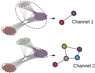
We investigate how multiple channels encodes the meaningful pooled graphs by visualizing the cluster assignments, and answer research question Q3. Figure 2 shows the two channels at layer 1, which are generated by learning and hard pooling a graph from COLLAB. Node colors represent the cluster memberships. We observe that these two channels encodes the distinct pooled structures of the input graph. To be specific, channel 1 extracts local structure of input graph, at which only the closely-connected nodes are assigned into a cluster. On the contrary, channel 2 preserves the global structure roles of nodes with blue and grey colors, which bridge the different communities. These channels encodes the inherently various characteristics of input graph, which makes the higher layers of MuchGNN being more informative for classifying graphs.
5 Conclusion
Motivated by the CNN architecture, we propose the multichannel framework named MuchGNN to learn the graph representation specifically. In detail, we design the graph convolutional filters to learn the various characteristics of nodes in the series of graph channels. The inter-channel graph convolutions are given to aggregate the entire graph channels and generate the one at the next layer. Experimental results show that we achieve state-of-the-art performance on the task of graph classification, and improve model robustness greatly. In the future works, we would apply MuchGNN to other tasks, such as the node classification and link prediction.
Acknowledgements
This work is, in part, supported by DARPA (#W911NF-161-0565) and NSF (#IIS-1750074, #IIS-1718840, and #IIS1900990). The views, opinions, and/or findings contained in this paper are those of the authors and should not be interpreted as representing any funding agencies.
@inproceedings{ijcai2020p188,
  title     = {Multi-Channel Graph Neural Networks},
  author    = {Zhou, Kaixiong and Song, Qingquan and Huang, Xiao and Zha, Daochen and Zou, Na and Hu, Xia},
  booktitle = {Proceedings of the Twenty-Ninth International Joint Conference on
               Artificial Intelligence, {IJCAI-20}},
  publisher = {International Joint Conferences on Artificial Intelligence Organization},
  editor    = {Christian Bessiere},
  pages     = {1352--1358},
  year      = {2020},
  month     = {7},
  note      = {Main track},
  doi       = {10.24963/ijcai.2020/188},
  url       = {https://doi.org/10.24963/ijcai.2020/188},
}
TY - CPAPER TI - Multi-Channel Graph Neural Networks AU - Zhou, Kaixiong AU - Song, Qingquan AU - Huang, Xiao AU - Zha, Daochen AU - Zou, Na AU - Hu, Xia T2 - Proceedings of the Twenty-Ninth International Joint Conference on Artificial Intelligence, IJCAI-20 PB - International Joint Conferences on Artificial Intelligence Organization PY - 2020 SP - 1352 EP - 1358 DO - 10.24963/ijcai.2020/188 UR - https://doi.org/10.24963/ijcai.2020/188 ER -Copied
Machine-readable versions of this paper, for tools and AI agents:





