
Detecting Adversarial Attacks via Subset Scanning of Autoencoder Activations and Reconstruction Error
Proceedings of the Twenty-Ninth International Joint Conference on Artificial Intelligence. Main track. Pages 876-882.
https://doi.org/10.24963/ijcai.2020/122
Keywords
- Data Mining: Big Data, Large-Scale Systems
- Computer Vision: Statistical Methods and Machine Learning
- Machine Learning: Deep Learning
Abstract
Reliably detecting attacks in a given set of inputs is of high practical relevance because of the vulnerability of neural networks to adversarial examples.
These altered inputs create a security risk in applications with real-world consequences, such as self-driving cars, robotics and financial services.
We propose an unsupervised method for detecting adversarial attacks in inner layers of autoencoder (AE) networks by maximizing a non-parametric measure of anomalous node activations.
Previous work in this space has shown AE networks can detect anomalous images by thresholding the reconstruction error produced by the final layer. Furthermore, other detection methods rely on data augmentation or specialized training techniques which must be asserted before training time. In contrast, we use subset scanning methods from the anomalous pattern detection domain to enhance detection power without labeled examples of the noise, retraining or data augmentation methods. In addition to an anomalous “score” our proposed method also returns the subset of nodes within the AE network that contributed to that score. This will allow future work to pivot from detection to visualisation and explainability. Our scanning approach shows consistently higher detection power than existing detection methods across several adversarial noise models and a wide range of perturbation strengths.
- [Beggel et al., 2019] Laura Beggel, Michael Pfeiffer, and Bernd Bischl. Robust anomaly detection in im- ages using adversarial autoencoders. arXiv preprint arXiv:1901.06355, 2019.
- [Berk and Jones, 1979] Robert H. Berk and Douglas. H. Jones. Goodness-of-fit test statistics that dominate the Kol- mogorov statistics. Zeitschrift fär Wahrscheinlichkeitsthe- orie und Verwandte Gebiete, 47:47-59, 1979.
- [Chen and Neill, 2014] Feng Chen and Daniel B. Neill. Non- parametric scan statistics for event detection and forecast- ing in heterogeneous social media graphs. In KDD '14, pages 1166-1175, 2014.
- [Chen et al., 2019] Jianbo Chen, Michael I Jordan, and Mar- tin J Wainwright. Hopskipjumpattack: A query-efficient decision-based attack. arXiv preprint arXiv:1904.02144, 3, 2019.
- [Davis and Goadrich, 2006] Jesse Davis and Mark Goadrich. The relationship between precision-recall and roc curves. In Proceedings of the 23rd international conference on Machine learning, pages 233-240. ACM, 2006.
- [Frosst et al., 2018] Nicholas Frosst, Sara Sabour, and Ge- offrey Hinton. Darccc: Detecting adversaries by recon- struction from class conditional capsules. arXiv preprint arXiv:1811.06969, 2018.
- [Goodfellow et al., 2015] Ian J. Goodfellow, Jonathon Shlens, and Christian Szegedy. Explaining and harnessing adversarial examples. CoRR, abs/1412.6572, 2015.
- [Krizhevsky et al., 2009] Alex Krizhevsky, Geoffrey Hinton, et al. Learning multiple layers of features from tiny im- ages. Technical report, Citeseer, 2009.
- [Kurakin et al., 2016] Alexey Kurakin, Ian J. Goodfellow, and Samy Bengio. Adversarial examples in the physical world. CoRR, abs/1607.02533, 2016.
- [LeCun et al., 1998] Yann LeCun, Léon Bottou, Yoshua Bengio, and Patrick Haffner. Gradient-based learning ap- plied to document recognition. Proceedings of the IEEE, 1998.
- [Madry et al., 2017] Aleksander Madry, Aleksandar Makelov, Ludwig Schmidt, Dimitris Tsipras, and Adrian Vladu. Towards deep learning models resistant to adversarial attacks. arXiv preprint arXiv:1706.06083, 2017.
- [McFowland et al., 2018] Edward McFowland, III, Sriram Somanchi, and Daniel B. Neill. Efficient Discovery of Heterogeneous Treatment Effects in Randomized Exper- iments via Anomalous Pattern Detection. ArXiv e-prints, March 2018.
- [McFowland III et al., 2013] Edward McFowland III, Skyler D. Speakman, and Daniel B. Neill. Fast gener- alized subset scan for anomalous pattern detection. The Journal of Machine Learning Research, 14(1):1533-1561, Jun 2013.
- [Meng and Chen, 2017] Dongyu Meng and Hao Chen. Mag- net: a two-pronged defense against adversarial examples. In ACM CCS'17, 2017.
- [Moosavi-Dezfooli et al., 2016] Seyed-Mohsen Moosavi- Dezfooli, Alhussein Fawzi, and Pascal Frossard. Deep- fool: a simple and accurate method to fool deep neural networks. In Proceedings of the IEEE CVPR'16, pages 2574-2582, 2016.
- [Neill, 2012] Daniel B. Neill. Fast subset scan for spatial pattern detection. Journal of the Royal Statistical Society (Series B: Statistical Methodology), 74(2):337-360, 2012.
- [Nicolae et al., 2018] Maria-Irina Nicolae, Mathieu Sinn, Minh Ngoc Tran, Ambrish Rawat, Martin Wistuba, Valentina Zantedeschi, Nathalie Baracaldo, Bryant Chen, Heiko Ludwig, Ian Molloy, and Ben Edwards. Adversarial Robustness Toolbox v0.7.0. CoRR, 1807.01069, 2018.
- [Papernot and McDaniel, 2016] Nicolas Papernot and Patrick D. McDaniel. On the effectiveness of defensive distillation. CoRR, abs/1607.05113, 2016.
- [Sakurada and Yairi, 2014] Mayu Sakurada and Takehisa Yairi. Anomaly detection using autoencoders with non- linear dimensionality reduction. In Proceedings of the MLSDA'14, page 4. ACM, 2014.
- [Samangouei et al., 2018] Pouya Samangouei, Maya Kabkab, and Rama Chellappa. Defense-gan: Protecting classifiers against adversarial attacks using generative models. arXiv preprint arXiv:1805.06605, 2018.
- [Schölkopf et al., 2001] Bernhard Schölkopf, John C Platt, John Shawe-Taylor, Alex J Smola, and Robert C Williamson. Estimating the support of a high-dimensional distribution. Neural computation, 13(7):1443-1471, 2001.
- [Szegedy et al., 2013] Christian Szegedy, Wojciech Zaremba, Ilya Sutskever, Joan Bruna, Dumitru Er- han, Ian J. Goodfellow, and Rob Fergus. Intriguing properties of neural networks. CoRR, abs/1312.6199, 2013.
- [Xiao et al., 2017] Han Xiao, Kashif Rasul, and Roland Vollgraf. Fashion-mnist: a novel image dataset for bench- marking machine learning algorithms. arXiv preprint arXiv:1708.07747, 2017.
- [Zhai et al., 2016] Shuangfei Zhai, Yu Cheng, Weining Lu, and Zhongfei Zhang. Deep structured energy based models for anomaly detection. arXiv preprint arXiv:1605.07717, 2016.
- [Zhou and Paffenroth, 2017] Chong Zhou and Randy C Paf- fenroth. Anomaly detection with robust deep autoen- coders. In ACM SIGKDD'17, pages 665-674. ACM, 2017.
References were extracted automatically from the PDF and may contain errors.
Full text extracted automatically from the PDF; figures, tables and equations may differ. The PDF is the version of record.
1 Introduction
Deep neural networks are susceptible to adversarial perturbations of their input data that can cause a sample to be incorrectly classified [Szegedy et al., 2013; Goodfellow et al., 2015; Kurakin et al., 2016]. These perturbations contain small variations in the pixel space that cannot be detected by a human but can change the output of a classifier.
The vulnerability of networks to adversarial examples implies a security risk in applications with real-world consequences, such as self-driving cars, robotics and financial services [Chen et al., 2019]. Detection of adversarial attacks is a key component to creating effective defense mechanisms.
∗Contact Author
Autoencoders (AE) are trained to re-create the input image by minimizing the reconstruction error (RE) of their output. Attack detection can be performed by looking at the distribution of the mean reconstruction error for clean and noised samples [Frosst et al., 2018]. Images with higher mean reconstruction error may be due to an adversarial perturbation of the input image which results in poorer reconstruction of the output. Since attacks are becoming increasingly sophisticated and coming from unknown diverse sources, it is not feasible to obtain labeled datasets of all possible attacks or build specific detection mechanisms for each type of attack. There are a variety of methods to make neural networks more robust to adversarial noise. Some require retraining of the model with adversarial examples [Goodfellow et al., 2015] or altering loss functions during the training step [Papernot and McDaniel, 2016].
In this paper, we build on subset scanning methods from the anomalous pattern detection literature [Neill, 2012; McFowland III et al., 2013]. We show these methods enhance the adversarial attack detection power of AEs in an unsupervised manner and without a priori knowledge of the attack or labeled examples. Anomalous pattern detection extends standard anomaly detection by searching for anomalous groups of records. Critically, these records may not appear anomalous when viewed individually. Subset scanning methods have been shown to succeed where other anomalous pattern detection heuristics may fail. "Top-down" methods look for globally anomalous signals (i.e., a high mean reconstruction error) and then sub-divide to find smaller, more anomalous groups of data points. These may fail if the true anomaly is not evident from global aggregates. "Bottom-up" methods look for individually anomalous signals (i.e., high reconstruction error at a single pixel) and then aggregate them into clusters. These may fail if the true anomaly is only evident by looking at groups of data points collectively. In contrast, subset scanning methods are designed to efficiently identify the most anomalous subset of data points -i.e., a group of pixels all with higher than expected reconstruction error. More details are provided in Section 3.
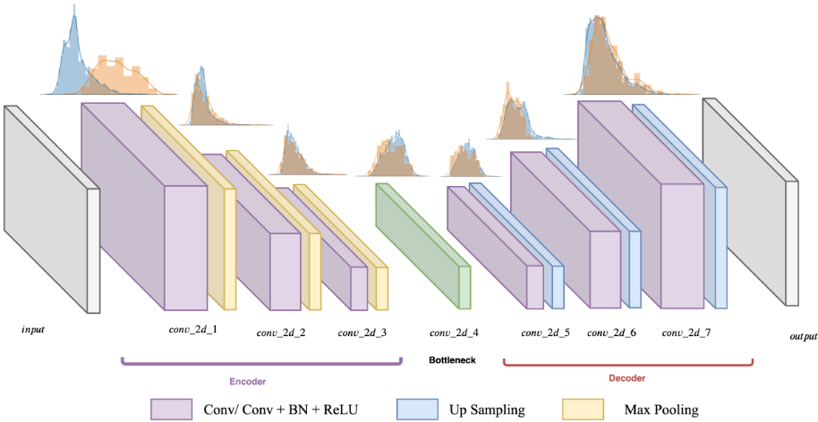
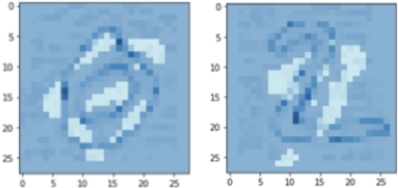
We claim three novel contributions of this work. First, we show how subset scanning methods can be applied to activations from internal layers of AE networks (see Figure 1). Second, we show this method can also be applied to the reconstruction error (pixel space) of the images which enables visualisations of how the adversarial perturbations of the input affects the output (see Figure 3). Third, we provide detection power results (AUC) for these proposed methods, baseline methods, and DefenseGan [Samangouei et al., 2018] for three commonly used image datasets and four different adversarial attacks (see Tables 2 and 3). Our scanning methods have higher detection power than DefenseGan for a wide range of perturbation strengths, ϵ. DefenseGan has comparable results on MNIST and F-MNIST when the perturbations are very large (ϵ = 0.15) but struggles to detect smaller perturbations.
2 RelatedWork
2.1 Adversarial Attack Detectors with Autoencoders and Generative Models
Several approaches have been used for adversarial attack detection with autoencoders and generative models, such as GANs [Samangouei et al., 2018] and variations of autoencoders [Beggel et al., 2019; Zhou and Paffenroth, 2017]. Since these methods can model training data distribution, these neural networks are an interesting option for adversarial attack detection. The majority of the methods discussed in literature require the training data to consist of normal examples only, such as denoising autoencoders [Meng and Chen, 2017]. The use of adversarial autoencoders by combining criterion of reconstruction error and likelihood in the latent space is discussed in [Beggel et al., 2019]. The authors also explored a retraining method to increase the separation in both latent and image space. [Zhou and Paffenroth, 2017] present an extension of denoising autoencoders that can work with corrupted data, where the network uses an anomaly regularizing penalty based on Lp-norms during training.The authors in [Zhai et al., 2016] used deep structured energy-based models to show that a criterion based on an energy score can lead to better results than the reconstruction error criterion. Defense-GAN [Samangouei et al., 2018] uses a generative adversarial trained model to encode the distribution of unperturbed images. The attack detection is performed using the mean square error of an image with its reconstruction formed from the generator as a metric to decide whether the image was perturbed.
Our proposed approach provides a way to quantify, detect, and characterize the data that are generated by various adversarial attacks. It does not rely on labeled examples, data augmentation or specialized training techniques which must be asserted before training time.
2.2 Adversarial AttackModels
There are several adversarial attack models discussed in the literature such as [Szegedy et al., 2013; Goodfellow et al., 2015; Moosavi-Dezfooli et al., 2016; Madry et al., 2017; Chen et al., 2019]. One way to classify these adversarial attacks is by their threat models, of which there are two main types: white-box and black-box. In the white-box approach, an attacker has complete access to the model, including its structure and trained weights. Several examples of whitebox attacks are used in this work such as Basic Iterative Method (BIM) [Kurakin et al., 2016], Fast Gradient Signal Method (FGSM) [Goodfellow et al., 2015], DeepFool (DF) [Moosavi-Dezfooli et al., 2016]. In the black-box approach, an attacker can only access the outputs of the target model. As an example of this modality, we use HopSkipJumpAttack [Chen et al., 2019]. For both threat models, the attacks can be targeted and untargeted. An untargeted attack perturbs the input to cause any type of misclassification, whereas the objective of a targeted attack is to modify the decision of the model to a specific target class. In this work, we focus only on untargeted adversarial attacks and show attack algorithms for both white and black box approaches.
FGSM uses the sign of the gradient at every pixel to determine the direction in which to change the corresponding pixel value. Given an image X, its corresponding true label ytrue and the cost function J(X, ytrue), the FGSM attack forms the adversarial sample (Xadv ) as:
BIM is an extension of FGSM where adversarial noise is applied multiple times iteratively with a small step size:
where N denotes the number of iterations, and β is a constant that controls the magnitude of the perturbations.
DF [Moosavi-Dezfooli et al., 2016] computes the optimal perturbation to perform a misclassification. The robustness of the affine classifier f, f(x) = wT x + b, for an input X is equal to the distance of the input to the hyper-plane that separates both classes. So the minimal perturbation to change the classifier decision is the orthogonal projection defined as:
HSJ is a decision-based attack that assumes access to predicted outputs only. HSJ works by performing a binary search to find the decision boundary, estimating the gradient direction at the boundary point, and then updating the step size along the gradient direction until perturbation is successful.
3 Subset Scanning for Anomalous Pattern Detection in Autoencoder's Activations
Subset scanning treats the pattern detection problem as a search for the "most anomalous" subset of observations in the data. Herein, anomalousness is quantified by a scoring function, F(S), which is typically a log-likelihood ratio statistic. Therefore, the goal is to efficiently identify S∗ = argmaxS F(S) over all relevant subsets of node activations within an autoencoder that is processing an image at runtime. The particular scoring functions F(S) used in this work are covered in the next sub-section.
Treating the detection problem as a subset scan has desirable statistical properties [Neill, 2012]. However, the exhaustive search over groups quickly becomes computationally infeasible due to the exponential number of subsets of records. Fortunately, a large class of scoring functions used in subset scanning satisfy the Linear Time Subset Scanning
(LTSS) property that enables exact and efficient maximization over all subsets of data without requiring an exhaustive search [Neill, 2012]. The LTSS property essentially reduces the search space from 2N to N for a dataset with N records while guaranteeing that the highest-scoring subset of records is identified.
3.1 Non-parametric Scan Statistics
This work uses non-parametric scan statistics (NPSS) that have been used in other pattern detection methods [McFowland III et al., 2013; McFowland et al., 2018; Chen and Neill, 2014]. Although subset scanning can use parametric scoring functions (i.e., Gaussian, Poisson), the distribution of activations within particular layers are highly skewed and in some cases bi-modal. Therefore, this work uses non-parametric scan statistics that make minimal assumptions on the underlying distribution of node activations.
As described in Algorithm 1, let there be M background images Xz included in DH0 . These images generate activations AH0 zj at each node Oj of the trained autoencoder. For example, if we take a 2D convolution layer from the AE that takes a single image of size (32, 32, 3) with 16 filters and 3 × 3 kernel size, we will have (32 ∗ 32 ∗ 16) nodes. Let Xi (not in DH0 ) be a test image under evaluation. This image creates activations Aij at each node Oj. The p-value, pij, is the proportion of background activations AH0 zj greater than the activation induced by the test image Aij at node Oj. [McFowland III et al., 2013] extended this notion to p-value ranges such that pij is uniformly distributed between pmin ij and pmax ij . This current work makes a simplifying assumption to only consider a range by its upper bound, defined as:
We convert the test image Xi to a vector of p-values pij of length J = |O|, the number of nodes in the network under consideration. The key assumption is that under the alternative hypothesis of an anomaly present in the activation data, then at least some subset of the activations SO ⊆ O will systematically appear extreme. We now turn to non-parametric scan statistics to identify and quantify this set of p-values.
The general form of the NPSS score function is
where N(S) represents the number of empirical p-values contained in subset S and Nα(S) is the number of p-values less than (significance level) α contained in subset S. In the above function, the α level defines a threshold, which pvalues can be compared against. Specifically, we calculate the number of pmax ij that fall below the threshold.
Moreover, it has been shown that for a subset S consisting of N(S) empirical p-values, E [Nα(S)] = N(S)α [McFowland III et al., 2013]. We assume an anomalous process will create some S where the observed significance is higher than the expected, Nα(S) > N(S)α, for some α.
There are well-known goodness-of-fit statistics that can be utilized in NPSS [McFowland et al., 2018]. In this work we use the Berk-Jones test statistic [Berk and Jones, 1979]:
x) log 1-x 1-y between the observed and expected proportions of significant p-values. Berk-Jones can be interpreted as the log-likelihood ratio for testing whether the p-values are uniformly distributed on [0, 1] as compared to following a piecewise constant alternative distribution, and has greater power than any weighted Kolmogorov statistic.
3.2 Efficient Maximization of NPSS for a Single Image
The NPSS evaluates the anomalousness of a subset of node activations for any given input. However, discovering the most anomalous subset from all the 2J possible subsets is computationally intensive even for a moderately sized J. To enable efficient and exact maximization of the NPSS score function over the exponentially many subsets, we exploit the linear-time subset scanning property (LTSS) [Neill, 2012] of the function. For any given subset of nodes SO, a score function F(S), and a priority function G(Oj), the LTSS property guarantees that a subset consisting of the "top k" priority nodes maximizes F(S) for some k in 1 . . . J.
For NPSS, the priority function is the proportion of pvalues that are less than α. However, because we are scoring a single image there is only one p-value at each node and hence the priority of a node is either 1 (when the p-value is less than α) or 0 (otherwise). Therefore, for a given fixed α threshold, the most anomalous subset consists of all and only the nodes with p-values less than α.
To maximize the scoring function F(S) = maxα Fα(S) over all α values, we sort all the Oj nodes by their p-values in ascending order. We then score successively larger subsets by including the node with the next-largest p-value at each step, starting with the node with the smallest p-value first. The largest score obtained from these J subsets is guaranteed to be the highest scoring subset according to the LTSS property. The pseudo-code for subset scanning over autoencoder activations is described in Algorithm 1.
4 Experimental Setup
We study the performance of our proposed approach over two experiments. First, we apply our detection method over nodeactivations from individual internal layers of the AE network (convolutional, batch normalization, max-pooling, and up-sampling) and analyze the detection power in each layer. Second, we apply the subset scanning method on the reconstruction error of the AE network. As baselines, we use the detection capabilities of the autoencoder's mean reconstruction error distributions [Sakurada and Yairi, 2014] and OneSVM [Sch¨olkopf et al., 2001] for the autoencoder reconstruction error space analysis. We also compare our results with the state-of-the-art detection method Defense-GAN [Samangouei et al., 2018].
4.1 Autoencoders Training and Datasets
We train the same autoencoder architecture (4385 parameters) for both F-MNIST [Xiao et al., 2017] and MNIST [LeCun et al., 1998]; a similar structure was used (52975 pa- Algorithm 1. Pseudo-code for subset scanning over autoencoder activations.
input : Background set of images: Xz ∈ DH0 , Evaluation Image: Xi, training dataset, αmax. output: S∗E Score for Xi 1 AE ← TrainNetwork (training dataset); 2 AEy ← Some flattened layer of AE; 3 for z ← 0 toM do 4 for j ← 0 to J do 5 AH0 zj ←ExtractActivation (AEy, Xz) 6 for j ← 0 to J do 7 Aij ←ExtractActivation (AEy, Xi) pij = ∑Xz∈DH0 I(Azj>=Aij)+1 M+1 ; 8 p∗ij = {y < αmax ∀ y ⊆ pij}; 9 psij ←SortAscending (p∗ij ); 10 for k ← 1 to J do 11 S(k) = {py ⊆ psij ∀y ∈ {1, . . . , k}}; 12 αk =max(S(k)); 13 F(S(k)) ←NPSS (αk, k, k); 14 k∗ ← argmaxF(S(k)); 15 α∗ = αk∗; 16 S∗ = S(k∗ ); 17 return S∗ , α∗ , and F(S∗ )rameters) for CIFAR-10 [Krizhevsky et al., 2009], with additional Batch Normalization layers and input size and depth variations. The encoder comprises three convolutional layers, each with relu activations, and a maxpooling layer after every convolutional layer. The decoder comprises four convolutional layers, each with relu activations except the final layer which uses a sigmoid. Each consecutive pair of convolutional layers is interspersed with an upsampling layer. We train the autoencoder by minimizing the binary cross-entropy of the decoder output and the original input image using an adadelta optimizer for 100 epochs. Furthermore, we train the autoencoder with different levels of data poisoning, 100% of clean samples, 1% of adversarial samples, and 9% of adversarial samples. For this experiment, we use BIM as the attack and F-MNIST as the dataset.
For all experiments, M = |DH0 | = 7000 of the 10000 validation images and we used them to generate the background activation distribution (DH0 ) at each of the activation nodes per each inner layer. These images form our expectation of "normal" activation behavior for the network. They were not used again. The remaining 3000 images were used to form a "Clean" (|C| = 1500) sample and an "Adversarial" (|A| = 1500) noised sample. The set A only contains images that were successfully noised by each type of adversarial attack.
4.2 Adversarial Noise Sample Generation
We generate several adversarial attacks (briefly introduced in Section 2.2) for our experiments. To generate the attacks, a standard Convolutional Neural Network was trained for each
(b)
| Layers | Clean Training | Noised (1%) F-MNIST | Noised (9%) F-MNIST | |||||||
|---|---|---|---|---|---|---|---|---|---|---|
| F-MNIST | MNIST | |||||||||
| BIM | FGSM | DF | HSJ | BIM | FGSM | DF | HSJ | BIM | BIM | |
| conv2d 1 | 0.964 | 0.974 | 0.965 | 0.859 | 1.0 | 1.0 | 0.999 | 1.0 | 0.909 | 0.823 |
| max pool 1 | 0.972 | 0.979 | 0.965 | 0.861 | 1.0 | 1.0 | 0.999 | 1.0 | 0.928 | 0.850 |
| conv2d 2 | 0.519 | 0.530 | 0.686 | 0.515 | 0.975 | 0.941 | 0.953 | 0.998 | 0.441 | 0.700 |
| max pool 2 | 0.500 | 0.513 | 0.634 | 0.451 | 0.855 | 0.809 | 0.837 | 0.906 | 0.424 | 0.693 |
| conv2d 3 | 0.500 | 0.507 | 0.481 | 0.478 | 0.382 | 0.384 | 0.443 | 0.617 | 0.470 | 0.469 |
| max pool 3 | 0.473 | 0.478 | 0.479 | 0.432 | 0.374 | 0.373 | 0.423 | 0.523 | 0.451 | 0.450 |
| conv2d 4 | 0.403 | 0.406 | 0.483 | 0.247 | 0.270 | 0.271 | 0.261 | 0.349 | 0.472 | 0.410 |
| up sampl 1 | 0.403 | 0.406 | 0.483 | 0.247 | 0.270 | 0.271 | 0.261 | 0.349 | 0.472 | 0.410 |
| conv2d 5 | 0.413 | 0.419 | 0.474 | 0.282 | 0.228 | 0.228 | 0.193 | 0.161 | 0.356 | 0.388 |
| up sampl 2 | 0.413 | 0.419 | 0.474 | 0.282 | 0.228 | 0.228 | 0.193 | 0.161 | 0.346 | 0.388 |
| conv2d 6 | 0.342 | 0.350 | 0.483 | 0.331 | 0.259 | 0.261 | 0.285 | 0.255 | 0.306 | 0.323 |
| up sampl 3 | 0.342 | 0.350 | 0.483 | 0.331 | 0.259 | 0.261 | 0.285 | 0.255 | 0.306 | 0.323 |
| conv2d 7 | 0.594 | 0.597 | 0.506 | 0.691 | 0.693 | 0.688 | 0.848 | 0.882 | 0.613 | 0.603 |
Table 1. Detection power for subset scanning over all layers (convolutional, max pooling and up-sampling) for both datasets under three different adversarial attacks. The noised columns refer to the autoencoder being trained with 1% and 9% BIM noised samples. Under different datasets and attacks, the same initial layers hold the highest detection power. For BIM and FGSM attacks ϵ = 0.01.
dataset. The test accuracies for these models are 0.992 for MNIST, 0.921 for F-MNIST and 0.903 for CIFAR. BIM and FGSM attacks have a hyperparameter ϵ parameter which controls how far a pixel is allowed to change from its original value when noise is added to the image. We use a value of ϵ = 0.01 in the scaled [0, 1] pixel space over 100 steps. DeepFool used the standard ϵ = 1e - 06 and 100 iterations. The HopSkipJump attack was iterated over 100 steps. All untargeted attacks were generated with the Adversarial Robustness Toolbox [Nicolae et al., 2018]. Experiment results are shown in Tables 1 and 3. For comparison with Defense-GAN in Table 2, we used the proposed ϵ values for FGSM attack in [Samangouei et al., 2018]. Smaller values of ϵ make the pattern subtler and harder to detect, but also less likely for the attacks to succeed in changing the class label to the target.
5 Results
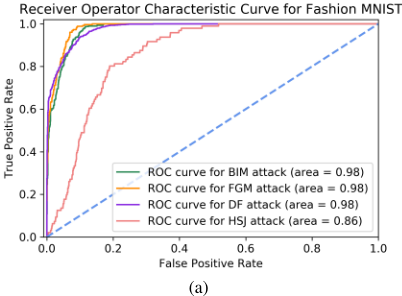
Detection power of the methods are reported by the Area Under the Receiver Operating Characteristic Curve (AUROC), which is a threshold independent metric [Davis and Goadrich, 2006] that rates the ability of the method to separate noised and clean images. Figure 2b shows the scores of the most anomalous subset of node-activations extracted from layer conv 2d 1 for F-MNIST clean images and F-MNIST images that have been (successfully) noised by various attacks. Figure 2a shows how these distributions are turned into ROC curves with their corresponding AUROC. This process is repeated for all layers in the AE and for MNIST images with results reported in Table 1. We observe across different experiments (noise models, and two proportions of noised samples during training), that the first layers (conv 2d 1 and max pooling 2d 1) maintain a high detection power (AUROC) between 0.86 to 1.0 depending on dataset and noise attack. Table 1 also shows the subset scanning detection power (above 0.82) for the cases where 1% and 9% of the samples are noised during the training stage of the autoencoder.
We compared detection power for our methods and Defense-GAN [Samangouei et al., 2018] for FGSM attacks over a range of ϵ values and data sets reported in Table 2. Our methods show substantial detection power advantages over Defense-GAN for subtle attacks. Furthermore, DefenseGAN struggled over all ϵ values in the more complex CIFAR10 data set. Table 3 shows the detection power of various methods over the reconstruction error space for different adversarial attacks. Our method performs better on MNIST than F-MNIST. One hypothesis for this is due to the autoencoder performance (loss for F-MNIST 0.284 and MNIST 0.095). If an autoencoder's loss is high, it is more difficult to separate between clean and noised samples in the reconstruction space because the most anomalous subset of reconstructed pixels of a clean image may be higher due to chance.
| Datasets | Epsilon (ϵ) | Detection Power (AUROC) | ||
|---|---|---|---|---|
| Defense-GAN | Subset Scan RE | Subset Scan AE | ||
| F-MNIST | 0.01 | 0.353 | 0.672 | 0.974 |
| 0.10 | 0.775 | 0.984 | 0.998 | |
| 0.15 | 0.884 | 0.995 | 0.999 | |
| 0.20 | 0.940 | 0.998 | 0.999 | |
| 0.25 | 0.969 | 0.999 | 0.999 | |
| MNIST | 0.01 | 0.234 | 0.983 | 1.0 |
| 0.10 | 0.914 | 0.999 | 1.0 | |
| 0.15 | 0.975 | 0.999 | 1.0 | |
| 0.20 | 0.989 | 1.0 | 1.0 | |
| 0.25 | 0.998 | 1.0 | 1.0 | |
| CIFAR | 0.10 | 0.410 | 0.600 | 0.755 |
| 0.15 | 0.425 | 0.710 | 0.903 | |
| 0.20 | 0.435 | 0.813 | 0.971 | |
| 0.25 | 0.446 | 0.889 | 0.993 | |
| 0.30 | 0.503 | 0.935 | 0.997 | |
| Datasets | Attacks | Detection Power (AUROC) | ||
|---|---|---|---|---|
| Ours RE | Mean RE | One-SVM | ||
| F-MNIST | BIM | 0.698 | 0.641 | 0.478 |
| FGSM | 0.672 | 0.630 | 0.497 | |
| DF | 0.599 | 0.477 | 0.534 | |
| HSJ | 0.956 | 0.935 | 0.546 | |
| MNIST | BIM | 0.998 | 0.751 | 0.624 |
| FGSM | 0.983 | 0.725 | 0.624 | |
| DF | 0.992 | 0.574 | 0.637 | |
| HSJ | 0.999 | 0.619 | 0.537 | |
Finally, subset scanning under the reconstruction error space is an interesting technique to inspect which pixels of the reconstructed image belong to the most anomalous subset. This highlights subset scanning methods returning both the anomalous score and which records in the data contributed to that score. An example of this is depicted in Figure 3 and leads to interesting future work.
6 Conclusions and FutureWork
In this work, we proposed a novel unsupervised method for adversarial attack detection with autoencoders and subset scanning. Current detection methods rely on data augmentation or specialized training techniques which must be asserted before training time. In contrast, we use subset scanning methods from the anomalous pattern detection domain to enhance detection power without labeled examples of the noise, re-training or data augmentation methods. Our scanning approach demonstrated consistently higher detection power than existing detection methods across several adversarial noise models and a wide range of perturbation strengths.
Moreover, applying our method over the reconstruction error space provides the pixels that belong to the most anomalous subset. Consequently, our approach is able to not only point out which image looks anomalous but also effectively detect and characterize the nodes that make the input a noised sample. Future work in this space will contribute to interpretability in addition to adversarial robustness.
@inproceedings{ijcai2020p122,
  title     = {Detecting Adversarial Attacks via Subset Scanning of Autoencoder Activations and Reconstruction Error},
  author    = {Cintas, Celia and Speakman, Skyler and Akinwande, Victor and Ogallo, William and Weldemariam, Komminist and Sridharan, Srihari and McFowland, Edward},
  booktitle = {Proceedings of the Twenty-Ninth International Joint Conference on
               Artificial Intelligence, {IJCAI-20}},
  publisher = {International Joint Conferences on Artificial Intelligence Organization},
  editor    = {Christian Bessiere},
  pages     = {876--882},
  year      = {2020},
  month     = {7},
  note      = {Main track},
  doi       = {10.24963/ijcai.2020/122},
  url       = {https://doi.org/10.24963/ijcai.2020/122},
}
TY - CPAPER TI - Detecting Adversarial Attacks via Subset Scanning of Autoencoder Activations and Reconstruction Error AU - Cintas, Celia AU - Speakman, Skyler AU - Akinwande, Victor AU - Ogallo, William AU - Weldemariam, Komminist AU - Sridharan, Srihari AU - McFowland, Edward T2 - Proceedings of the Twenty-Ninth International Joint Conference on Artificial Intelligence, IJCAI-20 PB - International Joint Conferences on Artificial Intelligence Organization PY - 2020 SP - 876 EP - 882 DO - 10.24963/ijcai.2020/122 UR - https://doi.org/10.24963/ijcai.2020/122 ER -Copied
Machine-readable versions of this paper, for tools and AI agents:





