The Price of Local Fairness in Multistage Selection

1 Introduction

The rise of algorithmic decision making in applications ranging from hiring to crime prediction [Perry et al., 2013] has raised critical concerns regarding potential unfairness towards groups with certain traits, supported by recent empirical evidences of discrimination [Lambrecht and Tucker, 2018; Larson et al., 2016]. This led to a fast-growing body of literature on what fairness in algorithmic decision making is and how to guarantee it (see related works below).

The existing literature typically considers one-shot decision processes whereby, from a set of features observed about an individual-one of them being a 'sensitive feature' based on which discrimination is defined-, one needs to decide whether or not to "select" him/her (where select can mean hire, grant a loan or parole, etc. depending on the context). The problem in this setting is how to learn a decision rule from past data that respects certain fairness constraints. In many applications, however, decisions are made in multiple stages. In hiring for instance, a subset of candidates is first selected for interview based on resume (or high-level candidate's information) and a final selection is then made from the subset of interviewed candidates. In police practices, there are often multiple stages of decisions with increasingly high levels of investigation of the individuals not released at the previous stage; as for instance in the famous stop-questionand-frisk practice by the New-York City Police Department.

∗The full version of this paper is available at the following link: https://hal.inria.fr/hal-02145071/document

A distinctive specificity of the multistage setting, besides the fact that decisions are made in multiple stages, is that in many cases additional features get known at later stages for the subset of individuals selected at earlier stages, but one needs to make the early-stage selection without observing those features. This raises a number of new questions that are fundamental to fair multistage selection. First, given that there are multiple layers of decisions, how should fairness be defined? In particular, should it be defined at each individual stage, on the final decision, or otherwise? Second, given that one has to make decisions with only partial information at early stages, how to make an optimal selection? Finally, given that the sensitive feature can be observed at different stages, is it better to observe the sensitive feature at earlier or later stages (for both fairness and utility)? This last question intuitively relates to recurrent public debates such as "should gender identification be removed from CVs?".

In this paper, we study the k-stage selection problem, in which there is a fixed limit (or budget) of candidates that can be selected at each stage (as is natural in the applications discussed). To tackle the questions above, we propose a simple model based on a probabilistic formulation in which we assume perfect knowledge of the joint distribution of features at all stages and of the conditional probability of being a desirable candidate conditioned on feature values. Based on this model, we are then able to make the following contributions.

We introduce two meaningful notions of fairness for the kstage setting: local fairness (the selection is fair at each stage) and global fairness (only the final selection needs to be fair).

These definitions extend classical group fairness notions for one-stage decision making (such as demographic parity or equal opportunity) to the multistage setting and they apply regardless of when the sensitive feature is observed (at first stage or later). We show that local fairness implies global fairness and we propose a linear formulation of the problem that allows us to compute the selection algorithm that maximizes precision while satisfying (local or global) fairness and per-stage budget constraints in expectation. As local fairness is a more restrictive condition, the precision of the optimal globally fair algorithm is naturally higher than for the locally fair algorithm. To capture this gap, we define the price of local fairness (PoLF ) as the ratio of the two and prove a simple upper bound-showing that imposing local fairness cannot be arbitrarily bad. We also define the notion of violation of local fairness (V oLF) to capture how far from locally fair the optimal globally fair algorithm is.

Finally, we conduct a numerical study in a two-stage setting using three classical datasets. Our results show that the PoLF can be large (up to 1.6 in some cases). This implies that in some cases, enforcing local fairness constraints can reduce the precision by 60% compared to a globally fair algorithm. The V oLF is also sometimes large (up to 0.6 in our experiments), which means that imposing only a global fairness constraint can be highly unfair at intermediate stages. We finally compare what happens when the sensitive feature is observed at the first stage or at the second stage. We find that the PoLF is generally higher when the sensitive feature is observed at the second stage; while conversely the V oLF is generally higher when the sensitive feature is observed at the first stage. These results show that, in most cases, it is possible to get at least approximate fairness at each stage and precision close to globally-fair optimal together; either by imposing local fairness if the sensitive feature is observed at first stage (where PoLF is small) or by hiding the sensitive feature at first stage and using a globally fair algorithm (which is close to locally fair since V oLF is then small).

Overall, our results provide intuitive answers towards better understanding fairness in multistage selection. To that end, we intentionally used the simplest model that captures the main features of a multistage selection problem and how an optimal selection algorithm is affected by the fairness notion considered and the time at which the sensitive feature is observed-rather than using a more practical but complex model. We believe that it is a good abstraction to start with, but we elaborate further on our model's limitations in Section 6. Due to space constraints, some details (proofs, additional formalization and experimental results) are omitted and can be found in the appendices of the full version.

Related Works

As mentioned earlier, there have been many recent works on defining fairness and constructing algorithms that respect those definitions for the case of one-stage decision making [Pedreshi et al., 2008; Dwork et al., 2012; Kleinberg et al., 2017; Hardt et al., 2016; Zafar et al., 2017; Chouldechova, 2017; Corbett-Davies et al., 2017; Kilbertus et al., 2017; Lipton et al., 2018]. Most of those works focus on classification and propose definitions of fairness based on equating some combinations of the classification outcome (true positives, true negatives, etc.). In this work, we focus on two classical notions of fairness for the one-shot classification setting: demographic parity (or disparate impact) and equal opportunity (or disparate mistreatment) [Hardt et al., 2016; Zafar et al., 2017]. There are also works on fairness in sequential learning [Joseph et al., 2016; Jabbari et al., 2017; Heidari and Krause, 2018; Valera et al., 2018]. The model in those papers is to sequentially consider each individual and make decision for them, but there is no notion of refining selection through multiple stages by getting additional features.

Closer to our work, a few papers investigate multistage classification/selection without fairness considerations [Senator, 2005; Trapeznikov et al., 2012]. [Schumann et al., 2019] model the interview decisions in hiring as a multi-armed bandit problem and consider getting extra features at a cost for a subset of candidates, but they do not have fairness constraints: they propose an algorithm for their bandit problem and show that it leads to higher diversity than other algorithms.

To the best of our knowledge, our paper is the first that proposes concrete fairness notions for multistage selection and algorithms to maximize utility under fairness constraints. The only other papers discussing fairness in the context of twostage or composed decision making are [Bower et al., 2017; Dwork and Ilvento, 2019], but they do not model additional features becoming available at the second stage for the subselected individuals, which is the key element of our analysis.

In recent work, [Kleinberg and Raghavan, 2018] consider the problem of selecting a subset of candidates to interview and show that under some condition, imposing diversity may increase utility when there is implicit bias. Their model, however, assumes no statistical knowledge of the features revealed at second stage, and they only maximize the sum of values of subsected candidates (effectively reducing to onestage). In contrast, we do not consider implicit bias but we do model the second-stage process. Interestingly, our optimal solution also introduces diversity at the first stage selection, but for different reasons.

2 Multistage Selection Framework

2.1 Basic Setting and Notation

Assume that there are n candidates, 1 each described by d features, and consider the following k-stage selection process. At the first stage, we observe some of the features x1, . . . , xd1 of the n candidates where d1 < d. We then select n1 of them that "pass" to the second stage. At the second stage, we observe some extra features of these n1 candidates xd1+1, . . . , xd2 (d1 < d2) that were not known at the previous stage. Using the features of both stages, we do a selection, from the n1 that passed the first stage of n2 ≤ n1 candidates that pass to the next stage, and so on. At the last stage k, we observe all dk = d features of the nk-1 candidates and select nk among those who passed the stage k - 1.

We assume that each candidate is endowed with a label y ∈ {0, 1}, which encodes whether the candidate is "good" or

1 We use the term candidates in a generic sense to refer to elements of the initial set that can be selected.

"bad" according to the purpose of the selection, i.e., if y = 1 we would like to have this candidate in our final selection, if y = 0 we would prefer not. The label y is not known until the end and is therefore not available to make the selection.

We assume that the decision maker knows the joint distribution of features and the conditional probability that expresses the probability that the candidate is "good" given all its features. We will denote by px1...xd = P(x1, . . . , xd) the probability to observe a specific realization of features and by py=1 x1...xd = P(y = 1|x1, . . . , xd) the probability that a candidate is good (y = 1) given its features x1 . . . xd.

2.2 Probabilistic Selection and Budget Constraints

In the following, we will consider a class of selection algorithms that perform a probabilistic selection of candidates. Such an algorithm takes as an input a list of probability values p(i|i-1) x1...xdi for all stages i ∈ {1 . . . k} and all possible combination of features. Then, for each candidate that passed stage i - 1 and has features (x1 . . . xdi ), the algorithm selects this candidate for the next stage with probability p(i|i-1) x1...xdi , with the convention that everyone passes stage 0.

For each stage i, we define a binary predictor ˆ yi that is equal to 1 if the candidate is selected at stage i (by convention, ˆ y0 = 1 for all candidates). We assume that, on average, the number of candidates that can be selected by the algorithm at stage i is at most αin and exactly αkn for the last stage, with 1 ≥ α1 ≥ · · · ≥ αk. We denote by α-k = (α1, · · · , αk-1)T the selection sizes of the first k-1 stages.

2.3 Performance Metric

We measure the performance of a given selection algorithm in terms of precision. The precision is the fraction of the selected candidates that indeed were "good" for selection:

where the denominator is the number of selected candidates.

The choice of precision may seem arbitrary but it is in fact a very natural metric when the size of the final selection is fixed as in our setting. Indeed, maximizing precision is then equivalent to maximizing most other meaningful metrics as formalized in the next proposition.

Proposition 1. Assume that the selection size P(ˆ yk = 1) is fixed (to αk). Then maximization of precision is equivalent to maximization of true positive rate, true negative rate, accuracy and f1-score; and to minimization of false positive rate and false negative rate.

Additionally, there are many realistic k-stage selection processes for which precision can be used as a utility metric.

Example 1. A bank decides to whom it will give entrepreneur loans. The procedure is in two stages: at first, n candidates fill in an application form, and the first d1 features of each candidate are obtained. Some candidates are then invited for an interview which brings additional features of those candidate that the bank can use for its final decision of selecting n2 candidates. If the profit of giving a loan to a trustworthy candidate is cp and if a candidate that does not pay a loan costs cl, then the average gain can be written as:

In this example, cp, cl and selection size n2 are fixed. Hence, maximizing precision or utility is equivalent.

3 Fairness Notions inMultistage Setting

In this section, we propose new notions of fairness for the multistage selection problem. We assume that there exists, amongst all features that describe candidates, a sensitive feature xs that indicates whether or not a candidate belongs to a sensitive group that should not be discriminated against.

The literature has introduced multiple definitions of fairness for the single-stage setting (and it is worth mentioning that in most of the cases those fairness criteria cannot be satisfied simultaneously [Chouldechova, 2017]). The most relevant notions in the context of selection problems are Demographic Parity (DP) and Equal Opportunity (EO). We first recall the definition of these fairness criteria in the traditional setting of single-stage selection. We then extend them to the multistage setting by showing that there are essentially two relevant notions of fairness: local and global fairness.

3.1 Classical Fairness Notions in Single-Stage

Let ˆ y be a binary predictor that decides which candidates belong to the selection. The first fairness definition, widely known as demographic parity, states that the predictor ˆ y is fair if it is statistically independent from xs.

Definition 1 (Demographic Parity, DP). The binary predictor ˆ y satisfies DP with respect to xs if ˆ y and xs are independent:

DP does not take into account the actual label y. [Hardt et al., 2016; Zafar et al., 2017] argue that DP is not the most relevant notion of fairness in cases where we have ground truth on the quality of the candidates (which is our case since we assume statistical knowledge of the probabilities of labels). In such cases, one might want to be fair among the candidates that are worth selecting, a metric called Equal Opportunity [Hardt et al., 2016] (an equivalent notion called disparate mistreatment is proposed in [Zafar et al., 2017]):

Definition 2 (Equal Opportunity, EO [Hardt et al., 2016]). The binary predictor ˆ y satisfies EO with respect to xs if ˆ y and xs are independent given that y = 1:

In the remainder, we systematically consider DP and EO.

3.2 Local and Global Fairness inMultistage

Existing fairness notions apply to single-stage selection, where we have only one binary predictor ˆ y. In the case of kstage selection, we have k binary predictors ˆ y = (ˆ y1, . . . , ˆ yk). In this section, we develop different notions of fairness that extend existing notions to the k-stage selection setting.

We propose three definitions that we believe correspond to three reasonable notions of fairness. The high-level idea of each definition is depicted on Figure 1. For the sake of brevity of exposition, we present the formal definitions for the demographic parity criterion, the translation to EO (or to any other fairness notion) being straightforward.

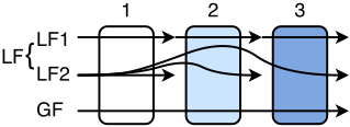
The first fairness notion, local fairness 1 (LF1), imposes that the selection be fair at every stage with respect to the set of candidates that reached that stage. In other words the selection of each stage i is fair with respect to the population that "passed" stage i - 1.

Definition 3 (Local Fairness 1, LF1). A k-stage selection algorithm satisfies LF1 if (for the case of DP), ∀i ∈ {1, · · · , k}:

The second fairness notion that we propose, local fairness 2 (LF2), prescribes that the selection should be fair at each stage with respect to the initial set of candidates.

Definition 4 (Local Fairness 2, LF2). A k-stage selection algorithm satisfies LF2 if (for the case of DP), ∀i ∈ {1, · · · , k}:

In the last definition, global fairness (GF), we allow the predictor ˆ yi to be unfair at each stage before the last, but we require the final decision ˆ yk to be fair with respect to the initial set of candidates.

Definition 5 (Global Fairness, GF). A k-stage selection algorithm satisfies GF if (for the case of DP):

Note that the above definitions can be adapted to EO by conditioning on y = 1 in all formulas.

3.3 Equivalence between LF1 and LF2

In the following proposition, we show that both notions of local fairness, LF1 and LF2 are equivalent. Therefore in the rest of the paper, we will simply name a multistage selection algorithm that satisfies LF1 (and thus LF2) as a being locally fair (LF). An algorithm satisfying the global fairness definition will be called globally fair (GF).

Proposition 2 (Relations between fairness notions). For both DP and EO:

1. A selection algorithm satisfies LF1 if and only if it satisfies LF2. We call such an algorithm locally fair (LF).
2. A locally fair selection algorithm is globally fair (GF).

4 UtilityMaximization as a Linear Program

Our goal is to find the binary predictors (ˆ y1, . . . , ˆ yk) corresponding to stages from 1 to k, respectively, that maximize precision while respecting budget and fairness constraints:

where functions fj(·) of the binary predictors correspond to the fairness constraints we impose. For instance, for a globally fair algorithm (DP) we have only one fairness constraint: f (ˆ y1, . . . , ˆ yk) = P (ˆ yk = 1|xs = 0) - P (ˆ yk = 1|xs = 1).

Using the assumption that the final stage size constraint is P (ˆ yk = 1) = αk we can write the precision as follows:

Using the notation introduced in Section 2.2, the probability P (ˆ yi = 1) that candidate passes stage i is

Hence, the constraints on the selection size P(ˆ yi = 1) ≤ αi for i < k and P(ˆ yk = 1) = αk can be expressed using (5).

The fairness constraints can be developed in the same manner, e.g., for the globally fair case (DP):

where ∀a ∈ {0, 1},

From (4), we see that the objective is not linear in the variables p(j|j-1) x1...xdj due to the product of probabilities. Similarly, we observe from (5) and (6) that the constraints are also not linear in these variables. However, we can show that by using the change of variables ˜ p(i|i-1) x1...xdi = ∏ij=1 p(j|j-1) x1...xdj , it can be made linear. This shows that it is possible to compute the variables p(j|j-1) x1...xdj that maximize precision (3) using a linear program (LP) (see details in Appendix A of the full version), which is key to applicability. It should be noted, however, that the number of variables in (LP) grows exponentially with the number of features.

To distinguish between the different notions of fairness, we will denote by U ∗LF (α-k, αk) and U ∗GF (α-k, αk) the value of the problem (LP)-i.e., the maximum utility-when the fairness constraints correspond to local and global fairness, respectively. Similarly, we will denote by U ∗ un (α-k, αk) the optimal precision value when no fairness constraint are imposed (we call it the unfair case).

4.1 Solution Properties wrt Budget Constraints

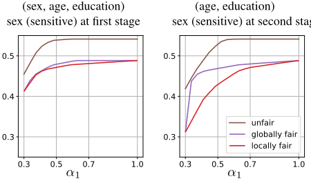
The selection sizes may be related to some budget or to some physical resources of our problem and are crucial parameters. As we show in the next proposition, the optimal utility values are monotonic and concave as functions of budget sizes α1, . . . , αk-1. This property can be useful for budget optimization and is illustrated as well on Figure 2.

Proposition 3 (Monotonicity and concavity). For U ∗ ∈ {U ∗LF , U ∗GF , U ∗ un } and any fairness constraints that can be expressed as linear homogeneous equations 2 (such as DP and EO), we have that U ∗ (α-k, αk) is

2 See details in Lemma 1 in Appendix A of the full version.

1. non-decreasing and concave with respect to α-k;
2. non-increasing with respect to αk.

Note that U ∗ can be concave or convex or none of the two with respect to αk, depending on the problem's parameters.

4.2 The Price of Local Fairness

We are now ready to define our central notion-the price of local fairness-that represents the price to pay for being fair at intermediate stages compared to a globally fair solution.

Definition 6 (Price of Local Fairness, PoLF). Let

It should be clear that the locally fair algorithm is more constrained than the globally fair. Thus, we have:

This implies that the values of PoLF(α-k, αk) are always larger than or equal to 1. Using only the final selection size αk, it is also possible to compute an upper bound as follows.

Proposition 4 (PoLF bound). For all (α-k, αk), we have:

For instance, if the final stage selection size is αk = 0.3 (as in our numerical examples), the globally fair algorithm can outperform the locally fair one by a factor at most 3.33. While this bound is probably loose, we will see in our numerical example that the PoLF can be as large as 1.6 on real data.

5 Empirical Analysis

In this section we implement 3 the optimization algorithms in order to capture tendencies on real datasets and to provide general insights. We consider the two-stage selection process, since it is the most easily interpretable. Thus, α-k = α1 and αk = α2. In our experiments we use three datasets: Adult [Dua and Graff, 2017], COMPAS [Larson et al., 2016] and German Credit Data [Dua and Graff, 2017]. We adapt these datasets to our two stage fair selection problem by leaving 6 features, binarizing them (see details in Appendix D of the full version) and artificially separating in two stages. We estimate the statistics px1...xd and py=1 x1...xd from data. We then use a linear solver for the linear program (LP) that gives us the optimal utility U ∗ (α1, α2) for the fair and unfair cases.

5.1 Analysis of the Price of Local Fairness

We consider three different scenarios: i) the sensitive attribute xs is observed at the first stage; ii) at the second stage; iii) never used in the selection process. We distinguish these three cases since it could happen that the use of the sensitive attribute xs in decision making is forbidden at some stages or even at all (by law or other conventions). Our aim is to compare how the price of local fairness behaves in every case.

Let us start with a simple example. We leave 5 features from the Adult dataset: sex, age, education, relationship and native country and consider the attribute sex as sensitive. Figure 2 then shows the values of U ∗ {un, GF, LF} (α1, α2) as a function of α1 for fixed α2 = 0.3 when using the features displayed on top of each subfigure at first stage and the rest at second stage. We make two important observations from this figure. First, the value of PoLF can be significant. From Figure 2-(right), we see that for α1 ≈ 0.33, the value of PoLF is about 1.3, meaning that the globally fair algorithm achieves 30% larger value of precision than the locally fair. Second, the gap between LF and GF algorithms is significantly larger when the sensitive attribute xs is observed at the second stage.

3 All codes are available at https://github.com/vitaly-emelianov/ multistage fairness/

To show that this behavior is significant we calculate the values of U ∗ {un, GF, LF} (α1, α2) for every possible combination X = {x1, . . . , x5} of 5 features out of 6 as decision variables (x1, x2 at first stage and x3, x4 at second stage), with one sensitive attribute xs = x5 that can be observed at the first stage or at the second stage or not observed at all, and for every possible (discretized) value of α1 ≥ α2. Due to space constraints we present our results only for the DP definition of fairness; we emphasize that the observations are robust among the three datasets and the two fairness notions (DP and EO) (see Appendix C for additional results). Figure 3 shows the empirical cumulative distribution functions ˆ FPoLF (x) of the values of PoLF obtained. We observe that the price of local fairness is significantly lower when the sensitive attribute xs is revealed at the first stage compared to the case where it is revealed later. This is consistent with the observation made on Figure 2. A possible interpretation is that the LF algorithm has to make a conservative decision at the first stage and therefore cannot perform well compared to the GF algorithm that is able to compensate (when the sensitive feature xs is observed) for the unfair decisions that have been made at the first stage. It is worth mentioning that we have the same observation for a three-stage algorithm: the later we reveal the sensitive attribute, the higher the values of PoLF we obtain (see Appendix C.4).

5.2 Violation of Local Fairness

By definition, a globally fair algorithm can violate fairness constraints at intermediate stages. For a given budget constraints α1, α2, we define the violation of local fairness (V oLF) as the absolute value of the fairness constraint violation at the first stage for the optimal globally fair algorithm. For instance, for DP, this quantity equals:

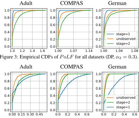
Figure 4 shows the empirical cumulative distribution function of violation of fairness ˆ FV oLF (x) for every value of α1 ∈ [α2; 1] and for every feature combination. We observe that the later the sensitive feature xs is revealed (or even not revealed), the more fair at intermediate stages the globally fair algorithm is. One possible explanation is that an algorithm that cannot observe the sensitive feature xs at the first stage has to be more "cautious" at every stage to be able to satisfy global fairness since the exact value of sensitive attribute xs is not available. This observation is again robust among different datasets and notions of fairness.

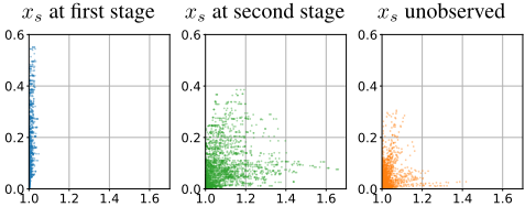
Finally, on Figure 5 we represent the joint distribution of PoLF and V oLF. As mentioned before, the globally fair algorithm is more unfair at the intermediate stages when the sensitive feature xs is observed from the beginning (left panel), however the price of local fairness we pay in this case is the smallest one. When the sensitive feature xs is observed at the second stage (middle panel) the globally fair algorithm is more locally fair compared to the previous case, but the value of PoLF is way larger. Finally, when xs is never observed (right panel) the globally fair algorithm is the "most locally fair" among all three settings. We finally observe that, while most points have either PoLF small (i.e., using a LF algorithm does not lose much) or V oLF small (i.e., the GF algorithm is almost locally fair), there exist some points-when the sensitive feature is observed at the second stage-where both PoLF and V oLF are large; i.e., imposing local fairness even approximately comes at a significant cost.

6 Conclusion

In this work we tackle the problem of multistage selection and the fairness issues it entails. We propose a stylized model based on a probabilistic formulation of the k-stage selection problem with constraints on the number of selected individuals at each stage that should hold in expectation. We introduce two different notions of fairness for the multistage setting: local (under two equivalent variants) and global fairness. Thanks to this framework, we show that maximizing precision under budget and fairness constraints can be done via linear programming, which enables for efficient computation as well as theoretical investigation. In particular, we analyze theoretically and empirically how the utility of locally and globally fair algorithms vary with selection budgets, and we find that globally fair algorithms can lead to non-negligible performance increases compared to locally fair ones.

One of the main findings of our work is that the stage at which the sensitive attribute is revealed greatly affects the difference between the performance of locally and globally fair algorithms: hiding the sensitive feature at early stages tends to make globally fair algorithm more fair at intermediate stages. While locally fair algorithms may be desirable, our results show that local fairness does not come for free. They also show that if a decision maker would like to encourage locally fair selection algorithms, there are essentially two choices: either hide the sensitive feature at the first stage or impose by rules the first stage to be fair.

Our model allows us to provide elegant insights into the fairness questions related to multistage selection, yet it does a number of simplifying assumptions that naturally restrict its direct applicability. First, our model ignores the issue that the selection probability at a stage depends on which candidates got selected at the previous stages; i.e., it implicitly makes the approximation that at each stage the number of candidates selected for each feature combination is equal to its expectation. In Appendix E of the full version, we show that this approximation becomes exact as n tends to infinity. Second, we assume perfect statistical knowledge of the joint distribution of features and label values, without bias. Third, we consider only discrete features and use a non-compact representation of the selection probabilities-this allows us to solve the exact selection problem by using an LP formulation. Relaxing these assumptions, in particular using a more compact representation of the selection algorithm (at the cost of a loss of precision) is an interesting direction of future work.

Acknowledgments

This work was supported in part by the French National Research Agency (ANR) through the "Investissements d'avenir" program (ANR-15-IDEX-02) and through grant ANR-16TERC0012; by the Alexander von Humboldt Foundation; and by a European Research Council (ERC) Advanced Grant for the project "Foundations for Fair Social Computing" funded under the European Union's Horizon 2020 Framework Programme (grant agreement no. 789373). The authors also thank Roland Hildebrand for helpful technical suggestions.