
Improving Law Enforcement Daily Deployment Through Machine Learning-Informed Optimization under Uncertainty
Proceedings of the Twenty-Eighth International Joint Conference on Artificial Intelligence. AI for Improving Human Well-being. Pages 5815-5821.
https://doi.org/10.24963/ijcai.2019/806
Keywords
- Special Track on AI for Improving Human-Well Being: AI benefits to society AI applications (Special Track on AI and Human Wellbeing)
- Special Track on AI for Improving Human-Well Being: Societal applications (Special Track on AI and Human Wellbeing)
Abstract
Urban law enforcement agencies are under great pressure to respond to emergency incidents effectively while operating within restricted budgets. Minutes saved on emergency response times can save lives and catch criminals, and a responsive police force can deter crime and bring peace of mind to citizens. To efficiently minimize the response times of a law enforcement agency operating in a dense urban environment with limited manpower, we consider in this paper the problem of optimizing the spatial and temporal deployment of law enforcement agents to predefined patrol regions in a real-world scenario informed by machine learning. To this end, we develop a mixed integer linear optimization formulation (MIP) to minimize the risk of failing response time targets. Given the stochasticity of the environment in terms of incident numbers, location, timing, and duration, we use Sample Average Approximation (SAA) to find a robust deployment plan. To overcome the sparsity of real data, samples are provided by an incident generator that learns the spatio-temporal distribution and demand parameters of incidents from a real world historical dataset and generates sets of training incidents accordingly. To improve runtime performance across multiple samples, we implement a heuristic based on Iterated Local Search (ILS), as the solution is intended to create deployment plans quickly on a daily basis. Experimental results demonstrate that ILS performs well against the integer model while offering substantial gains in execution time.
- [Amador et al., 2014] Sofia Amador, Steven Okamoto, and Roie Zivan. Dynamic multi-agent task allocation with spatial and temporal constraints. In Proceedings of the 2014 International Conference on Autonomous Agents and Multi-agent Systems, AAMAS '14, pages 1495-1496, Richland, SC, 2014. International Foundation for Au- tonomous Agents and Multiagent Systems.
- [Caplan et al., 2011] Joel M. Caplan, Leslie W. Kennedy, and Joel Miller. Risk terrain modeling: Brokering crim- inological theory and gis methods for crime forecasting. Justice Quarterly, 28(2):360-381, 2011.
- [Chase et al., 2017] Jonathan Chase, Jiali Du, Na Fu, Truc Viet Le, and Hoong Chuin Lau. Law enforcement resource optimization with response time guarantees. In IEEE Symposium Series on Computational Intelligence (SSCI) 2017, 2017.
- [Duvenaud et al., 2011] David K. Duvenaud, Hannes Nick- isch, and Carl E. Rasmussen. Additive Gaussian pro- cesses. In Proceedings of the Advances in Neural Infor- mation Processing Systems, pages 226-234, 2011.
- [Flaxman et al., 2015] Seth Flaxman, Andrew Gordon Wil- son, Daniel B. Neill, Hannes Nickisch, and Alexander J. Smola. Fast Kronecker inference in Gaussian processes with non-Gaussian likelihoods. In Proceedings of the ICML, pages 607-616, 2015.
- [Kennedy et al., 2011] Leslie W. Kennedy, Joel M. Caplan, and Eric Piza. Risk clusters, hotspots, and spatial intelli- gence: Risk terrain modeling as an algorithm for police re- source allocation strategies. Journal of Quantitative Crim- inology, 27(3):339-362, Sep 2011.
- [Lau et al., 2016] Hoong Chuin Lau, Zhi Yuan, and Aldy Gunawan. Patrol scheduling in urban rail network. An- nals of Operations Research, 239(1):317-342, 2016.
- [Levine, 2017] Ned Levine. CrimeStat: A Spatial Statistical Program for the Analysis of Crime Incidents, pages 381- 388. Springer International Publishing, Cham, 2017.
- [Lourenc ¸o et al., 2010] Helena R Lourenc ¸o, Olivier C Mar- tin, and Thomas Stützle. Iterated local search: Framework and applications. Handbook of Metaheuristics, 246:363- 397, 2010.
- [Malleson and Andresen, 2015] Nick Malleson and Mar- tin A Andresen. Spatio-temporal crime hotspots and the ambient population. Crime Science, 4(1):1-8, 2015.
- [Mukhopadhyay et al., 2016] Ayan Mukhopadhyay, Chao Zhang, Yevgeniy Vorobeychik, Milind Tambe, Kenneth Pence, and Paul Speer. Optimal allocation of police patrol resources using a continuous-time crime model. In De- cision and Game Theory for Security -7th International Conference, GameSec 2016, pages 139-158, 2016.
- [Murray et al., 2001] Alan T. Murray, Ingrid McGuffog, John S. Western, and Patrick Mullins. Exploratory spatial data analysis techniques for examining urban crimeimpli- cations for evaluating treatment. The British Journal of Criminology, 41(2):309-329, 2001.
- [Saisubramanian et al., 2015] Sandhya Saisubramanian, Pradeep Varakantham, and Hoong Chuin Lau. Risk based optimization for improving emergency medical systems. In Proceedings of the Twenty-Ninth AAAI Conference on Artificial Intelligence, AAAI'15, pages 702-708. AAAI Press, 2015.
- [Wilson and Weiss, 2012] Jeremy M Wilson and Alexander Weiss. A performance-based approach to police staffing and allocation. US Department of Justice Office of Com- munity Oriented Policing Services, 2012.
References were extracted automatically from the PDF and may contain errors.
Full text extracted automatically from the PDF; figures, tables and equations may differ. The PDF is the version of record.
1 Introduction
The question of safety and security is much discussed amidst an ever-increasing pressure on urban law enforcement agencies to respond to emergency incidents in a timely fashion. This is exacerbated by the need to economize on resources and reduce manpower requirements. An effective deployment is challenging, however, as it must be designed to account for the uncertain nature of future crime. In this work, we are concerned with improving emergency response in a national homeland security department through machine learninginformed optimization. We develop an algorithm that proposes a daily deployment plan, assigning law enforcement agents to patrol sectors in order to improve response times to emergency incidents.
∗Corresponding author: Hoong Chuin Lau (hclau@smu.edu.sg)
Optimization has been applied to law enforcement deployment, allocating officers to patrol rail stations [Lau et al., 2016] and deploying police cars to respond to crime incidents [Mukhopadhyay et al., 2016], for instance. The latter work solves a similar problem to this paper, but makes assumptions that are not practical in the real world scenario we are solving. Particularly, one car is sufficient to respond to all incidents in a geographic area, with the size of an area being malleable according to the demand. This is dependent on the assumption that travel time can be modeled using geographic distance, which is not realistic in our urban setting. Instead we use travel time prediction based on historical data [Chase et al., 2017], which means our deployment plans must use existing operational patrol regions, with multiple agents per region. Additionally, we address a wider variety of incidents than burglary crimes, including non-criminal emergency incidents, and thus we adopt a risk-based approach similar to [Saisubramanian et al., 2015], which improved response times in emergency medical systems. However, this work differs from ours by optimizing directly on historical data and allows the optimization formulation perfect knowledge of the sample space, an assumption that we remove. [Amador et al., 2014] allocates security agents to incidents as they occur, however, agents are allowed to change activity before completion of a task. This caveat is not acceptable for the real world problem we consider. The optimization model proposed in [Chase et al., 2017], addresses a similar problem context to this paper, but we are concerned not with the strategic problem of reducing manpower, but in deploying agents to reduce response time violations in daily (even hourly) operational settings. That work took a long-term planning approach, executed infrequently on historical data, aiming to minimize the agent supply subject to certain response time Quality of Service (QoS) requirements. It was possible that the optimization could 'look ahead', considering all incidents within the time range simultaneously. This means having the foresight to make dispatch decisions about earlier incidents in the light of later incidents, potentially achieving better response times than is realistic. The model presented in this paper introduces a significant realism improvement with a number of new constraints to ensure that the agent dispatched to an incident is the one that would be considered nearest if the incidents were considered strictly chronologically ('greedy dispatch').
Incident prediction is a significant challenge in law enforcement. Data sparsity, particularly for special occurrences such as public holidays, means that training deployment plans on a historical dataset may lack robustness to uncertainty. Previous methods include simple aggregation of historical demand [Wilson and Weiss, 2012; Malleson and Andresen, 2015], spatial (but not temporal) hot spot identification [Levine, 2017; Murray et al., 2001], and risk terrain modeling [Caplan et al., 2011; Kennedy et al., 2011]. [Mukhopadhyay et al., 2016] learns demand on a continuous time spatial grid, but only burglary incidents are modeled, with generated incidents used to design police deployment. In this paper, we develop a spatio-temporal generative machine learning incident prediction model to produce incidents to train our solution. Our model learns a grid of incidents but reflects a wide gamut of incident types, therefore we do not consider finegrained environmental features (e.g. liquor stores). Instead, we model incident types through clustering and learn each cluster's distributions for incident parameters such as duration and agent demand. We are unable to model directly the effect of a deployment on future crime patterns due to a lack of data, but a changing daily deployment plan will help to make agent locations unpredictable to criminals.
Our contributions are as follows: First, we propose a Sample Average Approximation (SAA) approach to solving a mixed integer linear deployment planning problem (MIP) using samples generated from the incident generation algorithm. Note that we allow for the high degree of stochasticity in the problem space by finding a single solution that gives a low risk of response time target violation on every sample, with the imperfect knowledge of the emergency dispatcher taken into account in the MIP model. Next, we propose an incident prediction and generation approach that learns from a rich historical incident dataset, and demonstrate its accuracy. Finally, to improve the scalability of the model, we implement an Iterated Local Search (ILS) heuristic and compare it to the MIP solution and show that our proposed approach is able to provide good solution quality and scalability.
2 Law Enforcement Resource Allocation
Agents are assigned to patrol predefined geographic regions, responding to incidents as they occur. Incidents arrive via emergency calls, and may correspond to a range of situations, from noise disturbances to murder. When an incident is logged, it is assigned a priority, 'urgent' or 'non-urgent', and the nearest available agent is dispatched. The agent should reach the incident location (the time of arrival is called the 'response time') within the limit defined by the QoS requirements. When incidents require more than one agent to attend, the nearest additional agents will be dispatched, although their response time need not be factored into the QoS. Agents attend an incident until it is resolved (the 'engagement time'), and only then are available to attend another incident. If the time from an incident occurring to the response time of the first agent is too large, an incident is marked as a failure. The objective, therefore, is to minimize the failure rate (or 'risk') across all incidents, by finding the optimal number of agents to allocate to each patrol region. An agent may serve any incident occurring in another region as long as it is the nearest available one at the time of call.
The problem space under consideration is highly stochastic, with daily variations in the number of incidents, with each incident having its own priority classification, occurrence time, engagement time, and agent demand. In this paper we improve on the current literature by modeling this uncertainty in two key ways. Firstly, we use machine learning to design an incident prediction method that generates sample sets of incidents that reflect the day-to-day variations in real historical incident data. This variation captures both the spatio-temporal variation in incident counts and their accompanying parameters, including different day types and incident types. We then formulate an MIP to find the number of agents required in each region to minimize response time failures, using SAA to find a solution that will be robust across multiple scenarios. Secondly, we model the fact that a real emergency dispatcher would not have advance knowledge of incidents. Even within a limited time horizon, the optimization model could dispatch an agent that is not the nearest available to ensure its availability for a subsequent incident, thus unrealistically improving the overall failure rate. Our optimization model forces the allocation of the nearest currently available agent regardless of future incidents. Whilst a human dispatcher may be able to make better decisions based on personal experience, this is difficult to model, so we take a pessimistic view, given the low failure tolerance of the scenario. In the following sections, we first present our MIP formulation that finds the optimal number of agents required in each patrol region, using SAA. We then outline the incident sample generation process that provides the sample set for the MIP. Finally we present the ILS method to find a balance between solution quality and runtime.
3 SAAOptimizationModel for Deployment Planning
We present our mathematical model as follows. The objective function (1), minimizes response time failures across all samples. We use the notion of a 'logical' law enforcement agent, denoted by i ∈ I, modeled as a binary variable, representing the decision that an agent is required in the patrol region assigned to agent i, li ∈ L. The maximum agents per region is given by |I|/|L|. Our allocation is therefore a decision to activate an 'agent' i, with the constraint that the activation across all samples must be the same (2), and the total number of active agents per sample is equal to the manpower supply specified as an input parameter (defined in (3), where Ymax is the agent supply). The notations used in this formulation are defined in Table 1.
When an incident r happens in sample s, the nearest drs agents (in terms of response time) will be assigned to attend.
The nearest agent is determined by the sum of the travel time Tli ,lr from the agent's patrol region li to the incident's location lr and the time for agent i to complete any incident it is currently attending. The response time requirement for the incident is assessed only for the first responder. Incident data is ordered chronologically by time of occurrence, so if q ≤ r, then tq ≤ tr . We assume that when an incident occurs, the ending time of currently occupied agents can be known, to ensure that even if all agents are occupied, the first available agent will be allocated to an incident. Without this assumption, it would be possible for an infeasibility to occur, since resource pre-emption is not allowed. This does not violate the 'no lookahead' restriction, as constraints ensure that the nearest available agent is always prioritized, so the dispatch cannot take advantage of this knowledge.
(5)
∑
q
yq,r i,s ∀i, q ≤ r, s
i,s = yr
Indices:
- i Agent index from set I and its patrol region li q, r, h Incident indices from set Rs and their location lq ,lr ,lh s Sample index from set S
Decision Variables:
- zr s Binary variable indicating if the response time target was met for request r, sample s
- yi Binary variable indicating if agent i is required
- yi,s Binary variable indicating if agent i is required for sample s
- yr i,s Binary variable indicating if agent i serves incident r in sample s
- yq,r i,s Binary variable indicating if i serves r after serving q in sample s
| Derived Variables: | |
|---|---|
| δr s ers ∆q,r s | Time when incident r is first attended in sample s Ending time for all agents serving r, sample s Binary indicator whether eq > tr , sample s |
| Parameters: | |
| Tli,lr | Travel time from location of agent i to location of request r |
| drs | Number of agents required by incident r, sample s |
| cr , Tc | Priority class of request r and the response time QoS target for that priority |
| trs | Start time of request r, sample s |
| gr s | Engagement time of request r, sample s |
| Ymax | The maximum number of agents to be allocated for each sample |
| M | An arbitrary large value |
Tli ,lr + trs +M · ∆q,r
s
Tli ,lr + trs +M · ∆q,r
s
Tli ,lr + eqs +M · (1 -∆q,r
s )
If multiple agents are dispatched to an incident, the response time is defined by the first agent to arrive at the scene.
Constraints (4) and (5) enforce this. δr s denotes the arrival time of the first agent for incident r, and Tli ,lr represents the travel time from the agent's location li to the incident location lr when r happens. Constraints (6)-(10) and (23)-(27) enforce 'greedy dispatch', assigning the nearest available agent. If all are busy, the first agent to become available is used. Similarly, (23) and (24) quantify the "alternative" response time if the incident r is assigned to agent i, extending the consideration across all incidents. (25) handles response for the special case of the first incident and (26)-(27) the last occurring incident. When an agent is attending an incident, it must remain at the incident for the entire duration required to service the request, it cannot be pre-empted to serve another request. Additionally, the number of agents required by an incident must be provided, without double-booking ((6) - (7) and (11) - (19)). Since incidents can be served by agents from different locations, the problem of planning the spatial and temporal resource supply becomes challenging. Constraints (20) - (21) determine the values of ers , which is the end time of serving incident r. If agent i attends incident r, this is the earliest time the agent is available to attend another incident. Response time success is calculated in constraint (22) where δr s is the arrival time for request r, with a responding time target of Tc for incidents of class c. If the response time minus the start time for an incident, r, exceeds the target, the binary variable, zr s = 1, indicating a failure. The objective function aims to minimize these failures.
3.1 Using the Solution for Deployment
The MIP model uses binary variables with corresponding patrol locations to represent the need for an agent to be active in that region. It is operationally infeasible to have literal agents who are on duty at certain times and inactive at others, thus a practical application would require a mapping of the roster of Ymax real agents to the binary decision variables with value 1. Likewise, while some of our numerical results consider a 24-hour period, this would in reality be split into two 12-hour shifts. These requirements can be achieved with a scheduling problem that fits within the law enforcement agency's existing operational structures, but is omitted due to space constraints and the simplicity of the model.
4 Incident Prediction and Generation
Incident prediction is used to generate sample incident sets to train our resource allocation model. Our deployment model generates fresh deployment plans on a regular basis (more precisely, daily), according to the features of the time period under consideration. Incident generation enables us to generate and experiment with unlimited training sets rather than relying on historical data. In the following we describe our machine learning approach, generating incidents spatiotemporally based on the historical incident dataset provided by a large urban law enforcement agency. This dataset spans a one-year duration and contains more than 200,000 incidents in total. For each incident, the data records the detailed information of the location (latitude and longitude), timestamp, type, priority, agents required, and engagement time.
4.1 Incident Count Prediction
We discretize the continuous space into patrol regions and the continuous time into intervals (in our case, 2-hour periods, chosen to reflect the current operational preference of agents being able to change patrol location every 2 hours). We also distinguish between different day types (specifically weekdays, weekends, and public holidays (PHs) of which we identify 3 distinct groups). Using the historical dataset, we obtain the incident count for each region and time interval for each day. We use a spatio-temporal Gaussian Process (GP) to generate a separate prediction model for the incident counts in each space-time division for each day type, incorporating side information ('features') into the GP kernel function [Flaxman et al., 2015]. These features include demographic and land use data indicating the proportion of a patrol region devoted to, for example, public transport links, as well as population density and housing types.
Let |S| denote the number of spatial grids and |T | the number of temporal intervals. For each type of incident, we wish to have a distribution of the count within each combination of |S| × |T|. Given a query tuple (x, y, t), where x, y and t represent the longitude, latitude and timestamp, respectively, we first hash it into a bin i that has features fi. Let (xi, yi) denote the centroid coordinates of the bin and ti the interval index. Given the tuple (xi, yi, ti, fi), we then wish to predict the number of incidents that occur in i. For simplicity, within each bin, the incidents are assumed to have uniform distribution.
Let i and j be two separate spatiotemporal "bins", the kernel function between i and j can be written as:
where ks and kt are the spatial and temporal kernel function, respectively. We can further incorporate side information f using the additive kernel feature [Duvenaud et al., 2011]:
for all features f ∈ f . A typical kernel function for the side information is the linear kernel.
Unlike techniques such as Linear, or Gradient Boosting, regression which provide point estimates, GP is a stochastic process that learns a multivariate distribution which can be sampled to generate incident count predictions that vary from sample to sample, increasing the richness of the resulting data.
4.2 Incident Parameters Prediction
In addition to the incident count, the overall demand and consequent availability of agents is also determined by the priority, engagement time, and number of agents required to attend an incident. Different incident types have different levels of priority and complexity (for example, a murder requires a faster response and more manpower and time to handle than a noise disturbance). We propose to calculate the complexity of an incident type using the linear combination:
complexity = 0.5˜ s + 0.5P90(s) + ¯ d, where ˜ s and P90(s) indicate median and 90th percentile engagement time, respectively, and ¯ d indicates mean agent demand, with Min-Max scaler applied to map the values to the range [0, 1].
The incident type is defined in the input dataset, but many incident types with higher priority and complexity are low in frequency, so we use K-Means++ Clustering to group similar (in priority and complexity) incident types. We identify 5 clusters and the proportion of incidents belonging to each cluster is calculated for each of the spatio-temporal bins. For each bin and cluster we learn distributions for each parameter. Engagement times follow the exponential distribution, we treat the priority parameter as a binomial distribution, and we model the agent demand as a multinomial distribution.
4.3 Incident Generation Algorithm
Given a day type and set of patrol regions, incident sets can be generated for training and then testing a deployment plan. The algorithm for generating a single sample is as follows:
- Given a set of patrol regions and a time range, sample the incident count distributions learned by the GP model for the day type under consideration, to generate an incident count for each spatio-temporal division. Round the count value to the nearest integer to obtain the number of incidents to be generated.
- For each incident, randomly assign it to an incident type cluster, using the historic incident cluster proportions for its spatio-temporal division as the probability of an incident being assigned to a cluster.
- Using the learned parameters for each cluster in each spatio-temporal division, sample values for engagement time, priority, and agent demand from their distributions for each incident. Start time in minutes is a randomly generated value within the 2-hour period.
Each day type is modeled separately, with a prediction model being trained for each. The proportion of incidents from each cluster by spatio-temporal division, and the learned parameters for each cluster, are also calculated for each day type individually. This ensures that the variations observed by day type are faithfully replicated. For example, in addition to changes in the incident counts, the proportion of high priority incidents in certain patrol regions changes significantly.
5 Iterated Local Search Heuristic
With the SAA formulation, the problem space increases rapidly with the number of samples, due to (2). To improve scalability, we employ the ILS heuristic technique [Lourenc¸o et al., 2010] to find a practical balance between solution quality and execution time. The ILS algorithm obtains an initial solution by greedy construction, and the ILS operation is repeatedly applied to move to better solutions, while reducing the risk of getting stuck in local optima. Once a local optimum is reached, the perturbation operation is applied to explore neighboring search regions, with the local search operation finding the local optimum within those regions. The greedy construction algorithm activates one agent at a time, allocating an agent to a patrol region if it improves the failure rate. This is repeated until Ymax agents have been allocated to patrol regions. From this baseline, we iteratively search for an improvement. For each ILS iteration, a perturbation operation randomly changes the location of p agents to form a new solution in an attempt to escape local optimality. We then carry out a local search, with each iteration of the search randomly changing each agent location in turn, keeping the change if the solution improves, until an iteration offers no improvements. One local search swap is equivalent to the perturbation operation where p = 1. When the local search terminates, if the resulting allocation offers superior performance to the current best allocation, it becomes the new best allocation. The next iteration continues with perturbation from this new best solution. The algorithm terminates when the maximum number of iterations, Tmax, is reached, and the allocation is returned as the proposed agent allocation. To find the failure rate of a proposed allocation, we execute a dispatch simulation [Chase et al., 2017], which chronologically responds to incidents using the proposed allocation according to the greedy dispatch principle and returns the percentage of incidents that fail the response time QoS across the test samples (this is also used to produce our numerical results).
6 Numerical Results
In this section, we present experimental results for our incident prediction and generation approach and SAA optimization and ILS algorithms for deployment planning. We use a year's real historical data (see section on Incident Prediction and Generation for details) to train and test our prediction and solutions. We implement our solution approach in Java, using the IBM CPLEX solver 1 to obtain results for our MIP model. We consider a geographic area containing 24 patrol regions over a 24-hour period, with response time targets of 15 and 30 mins for urgent and non-urgent incidents, respectively. For the sake of confidentiality, the experimental parameters have been designed specially for this paper and thus provide an effective test, but should not be taken as an indication of current practice. Therefore, calculated risk values provide meaningful comparisons between methods, but do not describe the current on-the-ground reality.
6.1 Comparison of ILS, MIP, and Greedy
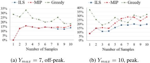
ILS aims to find a solution of competitive quality relative to the MIP, whilst achieving a significantly better runtime. The Greedy method is a baseline for the ILS, being the greedy construction algorithm from ILS. We set Ymax = 7 in Fig. 1a and Ymax = 10 in 1b during off-peak and peak 2-hour periods, respectively. The MIP is given an execution cutoff of 24 hours, with the best solution plotted for comparison. As the number of samples increases, the MIP execution time increases rapidly, with a single sample taking 84.05 seconds, but hitting the 24-hour cutoff for 3 samples and above. With 8 or more incident samples, the solutions diverge, as the MIP is no longer able to find a competitive solution within 24 hours. The Greedy solution is consistently worse than either method. With 10 agents, the MIP's runtime for a single sample is over 12 hours. The sample count is too small to guarantee a robust deployment plan, but the ILS algorithm is already providing a clear improvement. With the constraints added to improve realism and prevent lookahead, the MIP solution is not scalable enough, while the Greedy solution cannot compete on quality. Taking into account a balance of solution quality and execution time, the ILS is shown to provide a good solution.
1 https://www.ibm.com/analytics/cplex-optimizer
6.2 Evaluation of Incident Generation Algorithm
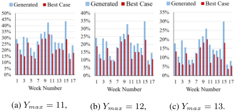
Incident generation allows for robust day-to-day planning when historical data is sparse, as well as sensitivity analysis to consider how a law enforcement agency would cope with changes in incident types, quantities, and patterns before they happen. This future-proofing is extremely important to law enforcement agencies. However, to be confident in the predictions, we must evaluate the accuracy of the algorithm output. Since incidents are complex with multiple parameters, count-based error metrics are inadequate, so we train the incident generator on one week of historical data, using the ILS algorithm to produce a deployment plan. This plan is evaluated over 17 weeks of test data as shown in Fig. 2. We also generate and evaluate a deployment plan for each week using the test data for both training and evaluation. This is therefore the 'best case scenario', the solution that would be produced given a perfectly accurate prediction. Thus, the bar height difference represents the error margin between prediction and reality. Even with a small amount of data used to train the incident generator, the average risk gap is approximately 5%, which is within acceptable margins for our application.
| Ymax = 11 | Ymax = 12 | Ymax = 13 | ||||
|---|---|---|---|---|---|---|
| Samples | Risk | Time (s) | Risk | Time (s) | Risk | Time (s) |
| 25 | 26.2% | 971 | 19.0% | 1123 | 14.1% | 1223 |
| 75 | 25.4% | 3090 | 18.9% | 3482 | 14.0% | 3928 |
6.3 Practical Solution Quality vs Execution Time
A deployment plan run daily must provide a good solution quickly enough to be executed at the start of a shift. We compute solutions using the incident data from the previous section to generate ILS solutions for combinations of incident samples and Ymax values, with the tradeoff between execution time and failure rate shown in Table 2. The number of samples generated has a significant impact on runtime as we increase from 25 to 75 samples, but the gain in solution quality is small. 25 samples are enough to capture the variations of the 1-week data used to train the incident generator, yet are robust across the 17 weeks of historical data. Additionally, the runtime of 15-20 minutes is excellent for a 24-hour planning period, compared to the hour-long runtime for 75 samples, without a large sacrifice in solution quality. This is a good result for ensuring practicality in the field.
7 Conclusions &FutureWork
In this work we introduced a deployment problem that seeks to generate daily patrol plans for a large, real urban law enforcement agency. Learning from historical data, we presented a probabilistic incident generation algorithm that learns spatio-temporal emergency incident patterns, taking into account different day types. We identified distinct incident type clusters and learn the distributions of each cluster's incident parameters. We presented an MIP model to robustly allocate law enforcement agents to patrol regions, using SAA across multiple generated incident samples. Given the scalability limitations of MIP solution methods, we employed an ILS-based heuristic algorithm that achieves good solution performance with a fast runtime, that outperforms both a simple greedy solution and the MIP (when the problem size becomes too large). Future work should improve the fidelity of the incident prediction model, to incorporate additional features, such as weather patterns and additional terrain features, e.g. hospitals, nightclubs, etc. Improvements to the deployment planner could incorporate a scheduling model for individual agents (as they are currently modeled as static binary variables), and performance enhancements for the local search heuristic. The greedy dispatch principle should also be examined, as techniques such as reinforcement learning may be able to design a practically-applicable dispatch strategy, that anticipates demand, and allows agents to dynamically redeployed to cover regions patrolled by occupied agents.
Acknowledgements
This research is funded by the National Research Foundation Singapore under its Corp Lab @ University scheme and Fujitsu Limited as part of the A*STAR-Fujitsu-SMU Urban Computing and Engineering Centre of Excellence.
@inproceedings{ijcai2019p806,
  title     = {Improving Law Enforcement Daily Deployment Through Machine Learning-Informed Optimization under Uncertainty},
  author    = {Chase, Jonathan and Nguyen, Duc Thien and Sun, Haiyang and Lau, Hoong Chuin},
  booktitle = {Proceedings of the Twenty-Eighth International Joint Conference on
               Artificial Intelligence, {IJCAI-19}},
  publisher = {International Joint Conferences on Artificial Intelligence Organization},
  editor    = {Sarit Kraus},
  pages     = {5815--5821},
  year      = {2019},
  month     = {8},
  note      = {AI for Improving Human Well-being},
  doi       = {10.24963/ijcai.2019/806},
  url       = {https://doi.org/10.24963/ijcai.2019/806},
}
TY - CPAPER TI - Improving Law Enforcement Daily Deployment Through Machine Learning-Informed Optimization under Uncertainty AU - Chase, Jonathan AU - Nguyen, Duc Thien AU - Sun, Haiyang AU - Lau, Hoong Chuin T2 - Proceedings of the Twenty-Eighth International Joint Conference on Artificial Intelligence, IJCAI-19 PB - International Joint Conferences on Artificial Intelligence Organization PY - 2019 SP - 5815 EP - 5821 DO - 10.24963/ijcai.2019/806 UR - https://doi.org/10.24963/ijcai.2019/806 ER -Copied
Machine-readable versions of this paper, for tools and AI agents:





