
Exact Bernoulli Scan Statistics using Binary Decision Diagrams
Proceedings of the Twenty-Eighth International Joint Conference on Artificial Intelligence. Main track. Pages 5737-5743.
https://doi.org/10.24963/ijcai.2019/795
Keywords
- Knowledge Representation and Reasoning: Tractable Languages and Knowledge compilation
- Uncertainty in AI: Exact Probabilistic Inference
Abstract
In combinatorial statistics, we are interested in a statistical test of combinatorial correlation, i.e., existence a subset from an underlying combinatorial structure such that the observation is large on the subset.
The combinatorial scan statistics has been proposed for such a statistical test; however, it is not commonly used in practice because of its high computational cost.
In this study, we restrict our attention to the case that the number of data points is moderately small (e.g., 50), the outcome is binary, and the underlying combinatorial structure is represented by a zero-suppressed binary decision diagram (ZDD), and consider the problem of computing the p-value of the combinatorial scan statistics exactly. First, we prove that this problem is a #P-hard problem. Then, we propose a practical algorithm that solves the problem. Here, the algorithm constructs a binary decision diagram (BDD) for a set of realizations of the random variables by a dynamic programming on the ZDD, and computes the p-value by a dynamic programming on the BDD. We conducted experiments to evaluate the performance of the proposed algorithm using real-world datasets.
- [Addario-Berry et al., 2010] Louigi Addario-Berry, Nicolas Broutin, Luc Devroye, Gábor Lugosi, et al. On combinato- rial testing problems. The Annals of Statistics, 38(5):3063- 3092, 2010.
- [Alon et al., 1995] Noga Alon, Raphael Yuster, and Uri Zwick. Color-coding. J. ACM, 42(4):844-856, 1995.
- [Arias-Castro et al., 2008] Ery Arias-Castro, Emmanuel J Candès, Hannes Helgason, Ofer Zeitouni, et al. Searching for a trail of evidence in a maze. The Annals of Statistics, 36(4):1726-1757, 2008.
- [Arias-Castro et al., 2011] Ery Arias-Castro, Emmanuel J Candes, Arnaud Durand, et al. Detection of an anomalous cluster in a network. The Annals of Statistics, 39(1):278- 304, 2011.
- [Bryant, 1992] Randal E Bryant. Symbolic boolean manipu- lation with ordered binary-decision diagrams. ACM Com- puting Surveys (CSUR), 24(3):293-318, 1992.
- [Cadena et al., 2017] Jose Cadena, Feng Chen, and Anil Vul- likanti. Near-optimal and practical algorithms for graph scan statistics. In Proceedings of the 2017 SIAM Interna- tional Conference on Data Mining, pages 624-632. SIAM, 2017.
- [Imai et al., 1999] Hiroshi Imai, Kyoko Sekine, and Keiko Imai. Computational investigations of all-terminal net- work reliability via bdds. IEICE transactions on funda- mentals of electronics, communications and computer sci- ences, 82(5):714-721, 1999.
- [Ishihata et al., 2010] Masakazu Ishihata, Yoshitaka Kameya, Taisuke Sato, and Shin-ichi Minato. An em algorithm on bdds with order encoding for logic-based probabilistic models. In Proceedings of 2nd Asian Conference on Machine Learning, pages 161-176, 2010.
- [Jerrum, 2003] Mark Jerrum. Counting, sampling and inte- grating: algorithms and complexity. Springer Science & Business Media, 2003.
- [Kawahara et al., 2017] Jun Kawahara, Takeru Inoue, Hi- roaki Iwashita, and Shin-ichi Minato. Frontier-based search for enumerating all constrained subgraphs with compressed representation. IEICE Transactions on Fun- damentals of Electronics, Communications and Computer Sciences, 100(9):1773-1784, 2017.
- [Knuth, 2009] Donald E Knuth. The art of computer pro- gramming: Bitwise tricks & techniques. Binary Decision Diagrams, 4, 2009.
- [Lugosi, 2017] Gábor Lugosi. Lectures on combinatorial statistics, 2017.
- [MacKinnon, 2009] James G MacKinnon. Bootstrap hy- pothesis testing. Handbook of Computational Economet- rics, 183:213, 2009.
- [Maehara et al., 2017] Takanori Maehara, Hirofumi Suzuki, and Masakazu Ishihata. Exact computation of influence spread by binary decision diagrams. In Proceedings of the 26th International Conference on World Wide Web, pages 947-956. International World Wide Web Confer- ences Steering Committee, 2017.
- [Minato, 1993] Shin-ichi Minato. Zero-suppressed bdds for set manipulation in combinatorial problems. In 30th ACM/IEEE Design Automation Conference, pages 272- 277. IEEE, 1993.
- [Minato, 2013] Shin-ichi Minato. Techniques of bdd/zdd: brief history and recent activity. IEICE TRANSACTIONS on Information and Systems, 96(7):1419-1429, 2013.
- [Qian et al., 2014] Jing Qian, Venkatesh Saligrama, and Yut- ing Chen. Connected sub-graph detection. In Artificial Intelligence and Statistics, pages 796-804, 2014.
- [Taylor and Tibshirani, 2015] Jonathan Taylor and Robert J Tibshirani. Statistical learning and selective infer- ence. Proceedings of the National Academy of Sciences, 112(25):7629-7634, 2015.
- [Weerahandi, 2013] Samaradasa Weerahandi. Exact statisti- cal methods for data analysis. Springer Science & Busi- ness Media, 2013.
References were extracted automatically from the PDF and may contain errors.
Full text extracted automatically from the PDF; figures, tables and equations may differ. The PDF is the version of record.
1 Introduction
Background and Motivation
Statistical test is one of the most important tools in decisionmaking under uncertainty. It evaluates how likely an observation occurs if a null hypothesis is true, and if it occurs very unlikely, we can reject the null hypothesis and accept the alternative hypothesis.
In this study, we consider a statistical test of "combinatorial correlation": Let V be a finite set, F ⊆ 2V be a set family that represents a combinatorial structure, and Xi ∈ R be a random variable for each i ∈ V . Our purpose is to show whether X = {Xi | i ∈ V } has a combinatorial correlation with respect to F with or not. Here, X has a combinatorial correlated with respect to F if there exists S ∈ F such that ∑i∈S Xi has a large value.
The combinatorial scan statistics [Lugosi, 2017] has been proposed for such a statistical test. Let xi ∈ R be an observation of Xi and let k = maxS∈F ∑i∈S xi. As the null hypothesis, we assume that each Xi follows an independent distribution. Then, under the null hypothesis, the p-value, which is the probability that an observation would be greater than or equal to the actual observation k, is given by
where
The random variable K is referred as the combinatorial scan statistics 1 . If the p-value is sufficiently small, we can reject the null hypothesis and conclude that there is a combinatorial correlation.
The combinatorial scan statistics has several applications [Addario-Berry et al., 2010]. However, it is not commonly used in practice because of its high computational cost (say, #P-hard; see also Theorem 2). [Arias-Castro et al., 2008] studied a test with respect to the paths of some class of graphs; however, they only discussed the asymptotic performance of simple tests based on the average. [Arias-Castro et al., 2011] studied a test with respect to the connected components in regular graphs; however, they did not discuss computational complexity. [Qian et al., 2014] studied an efficient algorithm for computing the positive elevated mean scan statistic with respect to the connected components of a graph. Here, the positive elevated mean scan statistics does not require computing the probability; hence it avoids the #P-hard computation. They proposed a method based on a semidefinite programming relaxation and rounding, which scales up to |V | ≤ 300 vertices; however, it has no theoretical guarantee about the approximation factor, which is not good for a statistical test. [Cadena et al., 2017] studied an efficient algorithm for computing non-parametric scan statistics for the small connected components (say, at most 10) of a graph. Here, the non-parametric scan statistics also avoids the #Phard computation. They employed a method based on the color coding technique [Alon et al., 1995], which scales up to components of size k ≤ 10; however, it is a randomized algorithm, which is not good for a statistical test, and its derandomization may be impractically expensive. It should be emphasized that all existing studies considered a particular type of combinatorial structures. Hence, these cannot be applied to more complicated (e.g., problem-specific-designed) combinatorial structures.
1 [Lugosi, 2017] simply referred to this as the "scan statistics."
In this study, to overcome the computational difficulty, we restrict our attention to the following problem setting.
- The number of regions, |V |, is small (e.g., ≤ 50).
- The outcome is binary, i.e., Xi ∈ {0, 1} for all i ∈ V .
- The feasible domain F is generic, i.e., given as an input of the problem.
This simple setting has not been considered yet but includes several important applications such as the test of regional differences of a presidential election result in the United States.
Problem Formulation and Our Contribution
Given our problem settings 1 and 2, we focus on the exact test [Weerahandi, 2013] that computes the p-value of Eq. (1) exactly (cf: non-exact tests employ asymptotic theory or MonteCarlo simulation to approximate the p-value). It is known that the exact test is preferred if there are only a small number of samples [MacKinnon, 2009]. Hence, it will fit our purpose.
Given our problem settings 1 and 3, we represent F as a binary decision diagram (BDD) [Bryant, 1992] or zerosuppressed binary decision diagram (ZDD) [Minato, 1993]. BDD/ZDD is a data structure that can represent a set family in a compact form. It has been applied in several problems such as paths, clusters, spanning trees, and so on. See [Minato, 2013] for a recent survey.
To summarize, our problem is the following.
Problem 1 (Exact Bernoulli Scan Statistics). We are given a finite set V , a ZDD (or BDD) D that represents a feasible domain F ⊆ 2V , and probability pi ∈ [0, 1] for each i ∈ V . Let Xi ∈ {0, 1} be random variable such that Xi = 1 with probability pi and Xi = 0 otherwise. The task is to compute the p-value of Eq. (1) exactly for a given k.
In this study, we first show that Problem 1 is #P-hard (Section 3). Then, we propose a practical algorithm to solve Problem 1 (Section 4).
Our main technical contribution is an algorithm that constructs a BDD for the following set family:
We refer this the weight family given a feasible domain F and k because each W ∈ Wk corresponds to a "binary weight vector" w = 1W ∈ {0, 1}V such that the optimal value of the linear maximization problemmaxS∈F ∑i∈S wi is at least k. We also refer its BDD the weight BDD. In the application to the combinatorial scan statistics, Wk corresponds to the set of realization of the random variable X such that the combinatorial scan statistics K of Eq. (2) is at least k. For a general F, computing the weight BDD is a non-trivial task. On the other hand, if F is represented by a ZDD, the weight BDD is obtained by a dynamic programming on the ZDD (Section 4.1).
Once we have the weight BDD, the probability
| name | meaning | complexity |
|---|---|---|
| union | S1 ∪ S2 | |D1||D2| |
| intersection | S1 ∩ S2 | |D1||D2| |
| complement | 2V \ S | |D| |
| select(i) | S.select(i) := {S ∈ S : i ∈ S} | |D| |
| add(i) | S.add(i) := {S ∪ {i} : S ∈ S} | |D| |
is efficiently obtained by a dynamic programming. Since this value equals to the p-value of Eq. (1), we can solve Problem 1 efficiently in the time proportional to the size of the weight BDD (Section 4.2).
As a side-product of having the weight BDD, we can also compute the post-selection inference [Taylor and Tibshirani, 2015] (Section 4.3).
We demonstrate the effectiveness of our algorithm by conducting experiments on real-world datasets (Section 5). We employ a family of connected subsets of a 48 contiguous US states and a 47 Japanese prefectures as a feasible domain F, and compute the scan statistics K of Eq. (2) and its p-value of Eq. (1) to test the localities of the changes of population, income, and GDP by state/prefecture. We also test the locality of the results of the 2016 US presidential election.
2 Preliminaries -BDD and ZDD
Let V be a finite set. A BDD [Bryant, 1992] is a directed acyclic graph D = (N(D), A(D)), where N(D) is the set of nodes containing a single root ρ and two terminals ⊤ and ⊥, and A(D) is the set of arcs. A path from the root to the ⊤ terminal corresponds to a subset of V in the following manner. Each non-terminal node α ∈ N(D) \ {⊤,⊥} is associated with an element i ∈ V of the underlying finite set (represented by α.label = i), and has exactly two out-going edges, called 1-arc and 0-arc. A node pointed by 1-arc and 0-arc of α are called 1-child and 0-child (denoted by α.1 and α.0), respectively. A path from the root to ⊤ represents a subset of V : the subset contains i ∈ V (resp. does not contain i) if-and-only-if the path contains the 1-arc (resp. 0-arc) of α such that α.label = i.
A BDD is ordered if V has a total order, and the element associated with α is smaller than that of the descendants of α. In the following, we only consider the ordered BDDs.
To make the diagram compact and canonical (i.e., uniquely determined), we make the following two assumptions called the BDD reduction rule.
- No two nodes have the isomorphic descendants.
- No node has the 1-arc and 0-arc that point to the same node.
An important property of BDD is that it admits efficient manipulations. We summarize the operations used in this study in Table 1.
ZDD [Minato, 1993] is a variant of BDD that employs the following assumptions called the ZDD reduction rule instead of the BDD reduction rule. Here, the first rule is the same as the BDD reduction rule, and the second rule is different.
- No two nodes have the isomorphic descendants.
- No node has the 1-arc that points ⊥.
For each application, we have to choose BDD or ZDD as a representation of a feasible domain. BDD is more suitable for a set family with many irrespective elements. For example, BDD is suitable for a family of the edge subsets of a graph that makes two specified vertices connected because a subset consists of a path between the vertices and other vertices that are irrespective to the connectivity [Imai et al., 1999; Maehara et al., 2017]. On the other hand, ZDD is more suitable for a sparse set family (i.e., each subset contains a small number of elements). For example, ZDD is suitable for a family of the edge subsets of a graph that forms a path between two specified vertices [Knuth, 2009].
3 #P-Hardness of the Problem
We prove that Problem 1 is #P-hard.
Theorem 2. Problem 1 is #P-hard and has no FPRAS unless NP = RP even if k = 2.
Proof. We reduce the #independent set problem 2 to Problem 1. Let G = (V (G),E(G)) be an instance of the #independent set problem (i.e., an undirected graph). We define F = {{u, v} : (u, v) ∈ E(G)}, p(u) = 1/2 for all u ∈ V (G) and k = 2. Note that the size of ZDD of F is bounded by O(∑S∈F |S|) because each path of the ZDD corresponds to a single set. In this case, this value is O(|E(G)|), which is linear in the size of the input.
The combinatorial scan statistics K in Eq. (2) satisfies K ≤ 1 if and only if for all (u, v) ∈ E(G), Xu +Xv ≤ 1 holds. In other words, {u ∈ V (G) : Xu = 1} forms an independent set of G. Therefore, 2|V (G)|P(K ≤ 1) = 2|V (G)| (1 - P(K ≥ 2)) is the number of independent sets of G.
This result implies that Problem 1 is hard for large instances. On the other hand, if the size of the instance is small (e.g., ≤ 50), there remains a hope to obtain a solution by a practically fast algorithm.
4 Exact Algorithm
In this section, we propose an algorithm to solve Problem 1. We assume that the feasible domain F is represented by a ZDD D because ZDD is more suitable than BDD to represent a sparse set family, such as paths and connected components, which are typical examples of underlying combinatorial structures of the combinatorial correlation tests. The algorithm can be easily adapted to the case that F is represented by a BDD.
Our goal is to construct a compact representation of the set family Wk in Eq. (3). We observe that this set family contains many irrespective elements because if W is in Wk, any superset of W is also in Wk. Therefore, we employ BDD to represent Wk.
2 The #independent set problem asks the number of independent set of a given graph G = (V (G), E(G)), where a subset I ⊆ V is an independent set if |I ∩ {u, v}| ≤ 1 for all (u, v) ∈ E(G). This problem is known to be #P-hard and has no FPRAS unless NP = RP [Jerrum, 2003].
Our algorithm consists of two steps: (1) construct a BDD of Wk, and (2) compute the p-value of the combinatorial scan statistics using the BDD of Wk. The second part uses a wellknown dynamic programming technique. Thus, the novelty of this study is in the first part.
4.1 Weight BDDConstruction
The algorithm is a dynamic programming on the ZDD D that manipulates the realized weight family Wk stored by BDDs.
Recall that each α ∈ N(D) induces a ZDD rooted by α, which represents a set family Fα ⊆ 2{α.label,...,|V |} . Note that Fα ̸= ∅ for all α ̸= ⊥ because of the reduction rule. Also, by the definition of ZDD, we have the following relations
where the union in Eq. (5) is a disjoint union (i.e., the first term and the second term are disjoint).
The algorithm maintains a BDD of the set family
for each α ∈ N(D) and ℓ ∈ {0, . . . , k}; namely, W[ρ][k] = Wk where ρ is the root of ZDD D, i.e., Fρ = F. For the initial condition, we have
Here, Eq. (9) follows because Fα ̸= ∅ since the ZDD is reduced. Eq. (10) follows by the definition. Eq. (11) follows because F⊥ = ∅. For the induction part, we have
These are computed in the reverse topological order of D. To verify this equation, we use the relations Eq. (5), Eq. (6), and Eq. (7). W ∈ W[α][l] if and only if there exists S ∈ Fα such that |S ∩ W| ≥ l. By Eq. (5), there are two cases: (1) S = S′ ∪ {α.label} for some S′ ∈ Fα.1, or (2) S ∈ Fα.0. In case (2), W is in W[α.0][l], which is captured by the first term of the right-hand side of Eq. (12). In case (1), there are two cases: (1-1) |S′ ∩W| ≥ l or (1-2) not. In case (1-1), W is in W[α.1][l], which is captured by the second term of the right-hand side of Eq. (12). In case (1-2), W satisfies that |S′ ∩W| = l - 1 and α.label ∈ W, which is captured by the third term of the right-hand side of Eq. (12). Consequently, the weight family Wk can be constructed by recursive evaluations of Eq. (12).
Our algorithm construct the weight BDD B = (N(B,A(B))) for the weight family Wk by dynamic programming on ZDD D. Let B[α][l] ∈ N(B) be a BDD node such that its corresponding set family is W[α][l]; B[ρ][k] represents Wk. Since all logical operations required in Eq. (12)
Algorithm 1 Construct the weight BDD B
Input: ZDD D = (N(D), A(D)) rooted by ρ
- 1: B[α][0] ← ⊤ for all α ∈ N(D) \ {⊥}
- 2: B[⊤][l] ←⊥ for all l ∈ {1, . . . , k}
- 3: B[⊥][l] ←⊥ for all l ∈ {0, . . . , k}
- 4: for α ∈ N(D) \ {⊤,⊥} in the reverse topological order of D do
- 5: B[α][l] ← B[α.0][l] ∪ B[α.1][l] ∪ B[α.1][l - 1].select(α.label) for all l ∈ {1, . . . , k}
- 6: end for
- 7: return the BDD induced by B[ρ][k] as B
Algorithm 2 Compute the probability P (Wk) on B
Input: BDD B = (N(B), A(B)) rooted by σ
- 1: P[⊤] ← 1, P[⊥] ← 0
- 2: for β ∈ N(B) \ {⊤,⊥} in the reverse topological order of B do
- 4: end for
- 5: return P[σ]
are supported by BDD operations as shown in Table 1, B can be constructed by recursive evaluations of Eq. (12) by BDD operations. For any B[α][l] and B[α′ ][l′ ], let B[α][l]∪B[α′ ][l′ ] return a BDD node representing W[α][l] ∪W[α′ ][l′ ] and also let B[α][l].select(α.label) return a BDD node representing W[α][l].select(α.label). Then, the overall algorithm for constructing the weight BDD is shown in Algorithm 1.
By Theorem 2, unless P = NP, the size of the weight BDD is not bounded by a polynomial in the size of the input (otherwise, by Algorithm 2 described below, we can solve Problem 1 in polynomial time). Therefore, Algorithm 1 is not a polynomial time algorithm. However, in practice, it works well on small size instances; see Section 5.2.
4.2 p-Value of Combinatorial Scan Statistics
Next, we show an algorithm to compute the p-value Eq. (1) exactly. As mentioned in Section 1, our goal is to compute P(Wk) defined in Eq. (4). This is performed by a standard dynamic programming technique [Ishihata et al., 2010].
Given the weight BDD B = (N(B), A(B)), the algorithm maintains a value P[β] that represents the probability of the set family represented by a BDD rooted by β ∈ N(B). For the initial condition, we have
For the induction part, we have
As same as Algorithm 1, we compute the values in the reverse topological order. Then, at the root node σ ∈ N(B), we have
Algorithm 2 shows the complete process. The runtime of the algorithm is proportional to the size of the BDD |B|.
4.3 Post-Selection Inference
Here, we show that Algorithm 1 can also be used for the postselection inference.
Suppose that we have observations xi for each i ∈ V . Then, we compute a combinatorial hotspot H ∈ argmaxS∈F ∑i∈S xi. Note that, in our case, H is obtained in linear time by a similar algorithm to Algorithm 2. The post-selection inference requires to compute the conditional probability
To compute this quantity, we construct BDDs of set family
for each l ∈ {0, . . . , kmax}, where kmax = maxS∈F |S|. This set family represents the set of realizations of X such that ∑i∈H Xi ≥ l. Note that this set family is Wk in the weight family for the singleton set family F = {H}. Therefore, we can use Algorithm 1 to construct the BDDs.
Once the BDDs are obtained, the set of realization of X such that H ∈ argmaxS∈F ∑i∈S Xi is obtained by
Using these families, the probability Eq. (16) is computed by
5 Experiments
We conducted experiments to evaluate the performance of the algorithm and to demonstrate applications to a real-world problem. All code was implemented in C/C++ (gcc 7.3.0 with the -O3 option) using SAPPOROBDD library 3 and TdZdd library 4 . All experiments were conducted on 64-bit Ubuntu 18.04.2 LTS with an Intel Core i7-7700K 3.6 GHz CPU and 16 GB RAM.
5.1 Experimental Setting
We apply our algorithm to test the locality of real-world observations: the population, income, and GDP changes of US and Japan, and the result of the 2016 US presidential election.
To test the locality, we employed a family of connected subsets of states/prefectures as a feasible domain F. Let GUS (resp. GJP ) be an undirected graph representing 48 contiguous states in North America (resp. 47 prefecture in Japan), and let F US ℓ (resp. F JP ℓ ) be a family of subsets of connected states (resp. prefectures) on GUS (resp. GJP ) of size ℓ. We constructed ZDDs DUS ℓ andDJP ℓ of F US ℓ andF JP ℓ , respectively, by the frontier-based construction method [Kawahara et al., 2017]. We omit the details of the construction time of the ZDDs since those are less than a second.
We obtained the estimated amounts of population, income, and GDP by state/prefecture from American FactFinder 5 and e-Stat 6 , official portal sites of US and Japanese governmental statistics, and computed the amount of change of each index. Table 2 shows information about the observations. We also obtained the result of the 2016 US presidential election from Wikipedia 7
3 https://github.com/takemaru/graphillion/tree/master/src/
SAPPOROBDD
4 https://github.com/kunisura/TdZdd
5 https://factfinder.census.gov/faces/nav/jsf/pages/index.xhtml
| Index | US | Japan |
|---|---|---|
| Population | 2012-2016 | 1976-2016 |
| Income | 2010-2017 | 2002-2014 |
| GDP | 1998-2017 | 2002-2014 |
| # observations | 32 | 67 |
5.2 Growth of theWeight BDD
Let WUS ℓ,k and WJP ℓ,k be the weight families of F US ℓ and F JP ℓ , respectively. Given ZDDs DUS ℓ and DJP ℓ , we constructed a shared weight BDD of {WUS ℓ,k | k ∈ {0, . . . , 48}} for ℓ ∈ {2, . . . , 48} and one of {WJP ℓ,k | k ∈ {0, . . . , 47}} for ℓ ∈ {2, . . . , 47}. Here, a shared BDD is a compact representation of multiple BDDs that shares their isomorphic subgraphs 8 . We denote the above shared weight BDDs by BUS ℓ and BJP ℓ , respectively.
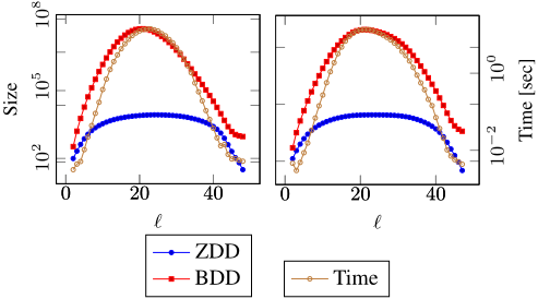
Figure 1 show that the relationship between the ZDD sizes |DUS ℓ | and |DUS ℓ |, the corresponding shared weight BDD sizes |BUS ℓ | and |BJP ℓ |, and their construction times. The size of the shared weight BDDs is 105 times larger than that of BDDs. The construction time of the shared weight BDD is proportional to its size. The longest construction time of the shard weight BDD of Japan is less than 10 seconds, and one of US is less than 13 minutes. Once we constructed BUS ℓ and BJP ℓ , we can compute the p-value of Eq. (1) in a few seconds.
Using the ZDD DUS ℓ and its shared weight BDD BUS ℓ , we can evaluate |F US ℓ | and |WUS ℓ,k | in time proportional to the sizes of the ZDD and BDD. For instance, |F US 20 | = 14,607,877,196 whereas |N(DUS ℓ )| = 8,966, and |WUS 20,20 | = 59,466,160,560,888 whereas |N(BUS ℓ )| = 38,901,120. This means that ZDDs/BDDs represent the set families very compactly, and without using them, it will be intractable to compute the p-values.
5.3 p-Values of Artificial Settings
We computed p-values of the following setting: For each ℓ ∈ {2, . . . , |V | - 1}, we observed X such that |X| = ℓ and its scan statistics K was also ℓ, that is, all states (or prefectures) with value 1 were connected. Then, we computed the p-value of the above observation X, where we set pi as the empirical probability ℓ/|V | for each i ∈ V . The p-value is the probability to observe 1s that form a connected subarea of size ℓ.
6 https://www.e-stat.go.jp/en
7 https://en.wikipedia.org/wiki/2016UnitedStatespresidentialelection
8 Many BDD libraries support shared BDDs and we can construct shared weight BDDs by running our algorithm using a such library.
| p-value | US dataset | Japan dataset | ||
|---|---|---|---|---|
| [0.0, 0.1) | 0 | (0.00%) | 9 | (0.79%) |
| [0.1, 0.2) | 1 | (0.21%) | 19 | (1.68%) |
| [0.2, 0.3) | 0 | (0.00%) | 17 | (1.50%) |
| [0.3, 0.4) | 7 | (1.44%) | 38 | (3.35%) |
| [0.4, 0.5) | 15 | (3.09%) | 53 | (4.67%) |
| [0.5, 0.6) | 149 | (30.66%) | 469 | (41.36%) |
| [0.6, 0.7) | 87 | (17.90%) | 121 | (10.67%) |
| [0.7, 0.8) | 10 | (2.06%) | 59 | (5.20%) |
| [0.8, 0.9) | 22 | (4.53%) | 102 | (8.99%) |
| [0.9, 1.0) | 195 | (40.12%) | 247 | (21.78%) |
| Total | 486 | 1134 | ||
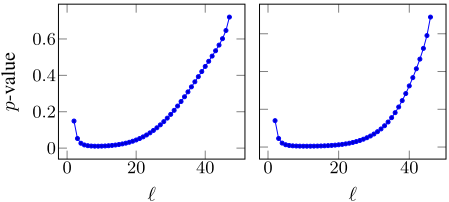
Figure 2 shows the relationship between ℓ and the p-value of US and Japan, respectively. The p-values of US with ℓ ∈ {4, . . . , 20} and those of Japan with ℓ ∈ {3, . . . , 28} are less than 0.05. This results infer that the probability of obtaining a connected subarea on Japan is smaller than one on US; it is natural because the width of GJP is narrower than that of GUS .
5.4 Population, Income, and GDP Changes in US and Japan
We computed the p-value of 36 and 67 observations shown in Table 2 given a feasible domain F US ℓ and F JP ℓ with changing ℓ ∈ {5, 10, 15, 20, 25, 30, 35, 40, 45}.
From each "amount of change" observation, we generated two types of "binary" observations: the first one is that a positive value (i.e., increasing) is 1 and a negative value (i.e., decreasing) is 0, and the second one is just opposite. To test a null hypothesis "the binary observation is generated from an i.i.d. distribution", we compute the p-value given the observation and a particular ℓ: the size of connected subareas. In this experiment, we set pi of observation X to the empirical probability |X|/|V | that is the ratio of 1s in the observation X. Consequently, we computed p-values of 32×2×9 = 572 hypotheses of US, and 67 × 2 × 9 = 1, 206 hypotheses of Japan.
Table 3 shows the histograms of p-values, where we omitted the results of trivial observations that consist only of 1s or 0s. 95% of the computed p-values of US and 88% of those of Japan are greater than 0.5, that is, most of observations have no locality with high probability.
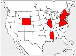
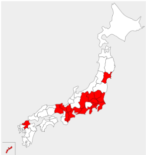
Figure 3 and 4 are the observations with the minimum pvalue of US and Japan, respectively. Figure 3 indicates that red states had negative population change in 2016, and its p-value with ℓ = 5 was 0.107. Figure 4 indicates that red prefectures had positive population change in 1999, and its pvalue with ℓ = 15 was 0.030. If we would test the above two hypotheses with significance level 0.05, the first one could not be rejected but the second one could be. Consequently, all 572 hypotheses of US could not be rejected because we exactly compute the p-value.
5.5 2016 US Presidential Election
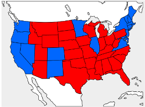
We computed the p-value of the results of the 2016 US presidential election. Figure 5 shows the result of the election: the red state indicates that Donald J. Trump won and the blue state indicates Hillary Clinton won. The number of red states is 29 and one of blue states is 19. Table 4 shows the p-values of red states and blue states with changing ℓ ∈ {5, 10, 15, 20, 25, 30}. All computed p-values are greater than 0.3, that is, it is difficult to conclude the results of the election have locality.
| ℓ | Blue States | Read States | ||
|---|---|---|---|---|
| K | p-value | K | p-value | |
| 5 | 5 | 0.879 | 5 | 0.999 |
| 10 | 10 | 0.382 | 10 | 0.954 |
| 15 | 13 | 0.682 | 15 | 0.806 |
| 20 | 16 | 0.691 | 20 | 0.604 |
| 25 | 19 | 0.528 | 25 | 0.335 |
| 30 | 19 | 0.555 | 29 | 0.346 |
Table 4: The combinatorial scan statistics K and its p-value of red and blue states with changing ℓ. There is no p-value significantly small.
6 Conclusion
We studied a problem of computing the p-value of the combinatorial scan statistics exactly. We restrict our attention to the case that the number of data points is moderately small, outcome is binary, and a feasible domain is represented by a ZDD. We first showed that the problem is #P-hard. Then, we proposed a practical algorithm that constructs a BDD for a set of the weight vectors by a dynamic programming on the ZDD, then computes the p-value by a dynamic programming on the BDD. We conducted experiments to evaluate the performance of the algorithm. The algorithm computes the pvalues in a minute when the feasible domain is the connected components of the graphs of the states in North America and the prefectures in Japan.
@inproceedings{ijcai2019p795,
  title     = {Exact Bernoulli Scan Statistics using Binary Decision Diagrams},
  author    = {Ishihata, Masakazu and Maehara, Takanori},
  booktitle = {Proceedings of the Twenty-Eighth International Joint Conference on
               Artificial Intelligence, {IJCAI-19}},
  publisher = {International Joint Conferences on Artificial Intelligence Organization},
  editor    = {Sarit Kraus},
  pages     = {5737--5743},
  year      = {2019},
  month     = {8},
  note      = {Main track},
  doi       = {10.24963/ijcai.2019/795},
  url       = {https://doi.org/10.24963/ijcai.2019/795},
}
TY - CPAPER TI - Exact Bernoulli Scan Statistics using Binary Decision Diagrams AU - Ishihata, Masakazu AU - Maehara, Takanori T2 - Proceedings of the Twenty-Eighth International Joint Conference on Artificial Intelligence, IJCAI-19 PB - International Joint Conferences on Artificial Intelligence Organization PY - 2019 SP - 5737 EP - 5743 DO - 10.24963/ijcai.2019/795 UR - https://doi.org/10.24963/ijcai.2019/795 ER -Copied
Machine-readable versions of this paper, for tools and AI agents:





