
Temporal Pyramid Pooling Convolutional Neural Network for Cover Song Identification
Proceedings of the Twenty-Eighth International Joint Conference on Artificial Intelligence. Main track. Pages 4846-4852.
https://doi.org/10.24963/ijcai.2019/673
Keywords
- Machine Learning: Deep Learning
- Multidisciplinary Topics and Applications: Information Retrieval
- Multidisciplinary Topics and Applications: Art and Music
Abstract
Cover song identification is an important problem in the field of Music Information Retrieval. Most existing methods rely on hand-crafted features and sequence alignment methods, and further breakthrough is hard to achieve. In this paper, Convolutional Neural Networks (CNNs) are used for representation learning toward this task. We show that they could be naturally adapted to deal with key transposition in cover songs. Additionally, Temporal Pyramid Pooling is utilized to extract information on different scales and transform songs with different lengths into fixed-dimensional representations. Furthermore, a training scheme is designed to enhance the robustness of our model. Extensive experiments demonstrate that combined with these techniques, our approach is robust against musical variations existing in cover songs and outperforms state-of-the-art methods on several datasets with low time complexity.
- [Bello, 2007] Juan Pablo Bello. Audio-based cover song re- trieval using approximate chord sequences: Testing shifts, gaps, swaps and beats. In International Society for Music Information Retrieval Conference, pages 239-244, 2007.
- [Bertin-Mahieux and Ellis, 2012] Thierry Bertin-Mahieux and Daniel PW Ellis. Large-scale cover song recognition using the 2d fourier transform magnitude. In International 4 see some examples on SHS100K-TEST https://www.dropbox. com/s/308z225hy31d3xa/RankList.xlsx?dl=0 Society for Music Information Retrieval Conference, pages 241-246, 2012. Link
- [Brown, 1991] Judith C Brown. Calculation of a constant q spectral transform. The Journal of the Acoustical Society of America, 89(1):425-434, 1991.
- [Chang et al., 2017] Sungkyun Chang, Juheon Lee, Sang Keun Choe, and Kyogu Lee. Audio cover song identification using convolutional neural network. In Workshop Machine Learning for Audio Signal Processing at NIPS, 2017.
- [Chen et al., 2018] Ning Chen, Wei Li, and Haidong Xiao. Fusing similarity functions for cover song identification. Multimedia Tools and Applications, pages 2629-2652, 2018.
- [Cheng et al., 2017] Yao Cheng, Xiaoou Chen, Deshun Yang, and Xiaoshuo Xu. Effective music feature ncp: En- hancing cover song recognition with music transcription. In Proceedings of the 40th International ACM SIGIR Con- ference on Research and Development in Information Re- trieval, pages 925-928. ACM, 2017.
- [Ellis and Poliner, 2007] Daniel PW Ellis and Graham E Po- liner. Identifying cover songs with chroma features and dy- namic programming beat tracking. In IEEE International Conference on Acoustics, Speech and Signal Processing, pages 1429-1432, 2007.
- [Fujishima, 1999] Takuya Fujishima. Realtime chord recog- nition for musical sound: a system using common lisp mu- sic. In ICMC, pages 464-467, 1999.
- [Grosche and Müller, 2012] Peter Grosche and Meinard Müller. Toward characteristic audio shingles for efficient cross-version music retrieval. In 2012 IEEE International Conference on Acoustics, Speech and Signal Processing (ICASSP), pages 473-476. IEEE, 2012.
- [He et al., 2015] Kaiming He, Xiangyu Zhang, Shaoqing Ren, and Jian Sun. Spatial pyramid pooling in deep con- volutional networks for visual recognition. IEEE trans- actions on pattern analysis and machine intelligence, 37(9):1904-1916, 2015.
- [He et al., 2016] Kaiming He, Xiangyu Zhang, Shaoqing Ren, and Jian Sun. Deep residual learning for image recog- nition. In Proceedings of the IEEE conference on computer vision and pattern recognition, pages 770-778, 2016.
- [Khadkevich and Omologo, 2013] Maksim Khadkevich and Maurizio Omologo. Large-scale cover song identification using chord profiles. In International Society for Music Information Retrieval Conference, pages 233-238, 2013.
- [Martin et al., 2012] Benjamin Martin, Daniel G Brown, Pierre Hanna, and Pascal Ferraro. Blast for audio se- quences alignment: a fast scalable cover identification. In International Society for Music Information Retrieval Conference, pages 529-534, 2012.
- [McFee et al., 2015] Brian McFee, Colin Raffel, Dawen Liang, Daniel PW Ellis, Matt McVicar, Eric Battenberg, and Oriol Nieto. librosa: Audio and music signal analysis in python. In Proceedings of the 14th python in science conference, pages 18-25, 2015.
- [Osmalsky et al., 2015] Julien Osmalsky, Jean-Jacques Em- brechts, Peter Foster, and Simon Dixon. Combining fea- tures for cover song identification. In International Society for Music Information Retrieval Conference, pages 462- -468, 2015.
- [Seetharaman and Rafii, 2017] Prem Seetharaman and Zafar Rafii. Cover song identification with 2d fourier transform sequences. In IEEE International Conference on Acous- tics, Speech and Signal Processing, pages 616-620, 2017.
- [Serrà et al., 2008] Joan Serrà, Emilia Gómez, Perfecto Her- rera, and Xavier Serrà. Chroma binary similarity and lo- cal alignment applied to cover song identification. IEEE Transactions on Audio, Speech, and Language Processing, 16(6):1138-1151, 2008.
- [Serrà et al., 2009] Joan Serrà, Xavier Serrà, and Ralph G Andrzejak. Cross recurrence quantification for cover song identification. New Journal of Physics, 11(9):093017, 2009.
- [Serrà et al., 2012] Joan Serrà, Holger Kantz, Xavier Serrà, and Ralph G Andrzejak. Predictability for music descrip- tor time series and its application to cover song detection. IEEE Transactions on Audio, Speech, and Language Pro- cessing, 20(2):514-525, 2012.
- [Silva et al., 2016] Diego F Silva, Chin-Chin M Yeh, Gus- tavo Enrique de Almeida Prado Alves Batista, Eamonn Keogh, et al. Simple: assessing music similarity using subsequences joins. In International Society for Music In- formation Retrieval Conference, pages 23-29, 2016.
- [Silva et al., 2018] Diego Furtado Silva, Felipe Vieira Fal- cao, and Nazareno Andrade. Summarizing and comparing music data and its application on cover song identification. In International Society for Music Information Retrieval Conference, pages 732-739, 2018.
- [Simonyan and Zisserman, 2015] Karen Simonyan and An- drew Zisserman. Very deep convolutional networks for large-scale image recognition. In International Confer- ence on Learning Representations, 2015.
- [Tzanetakis et al., 2003] George Tzanetakis, Andrey Er- molinskyi, and Perry Cook. Pitch histograms in audio and symbolic music information retrieval. Journal of New Mu- sic Research, 32(2):143-152, 2003.
- [Wang et al., 2017] Peng Wang, Yuanzhouhan Cao, Chun- hua Shen, Lingqiao Liu, and Heng Tao Shen. Temporal pyramid pooling-based convolutional neural network for action recognition. IEEE Transactions on Circuits and Systems for Video Technology, 27(12):2613-2622, 2017.
- [Xu et al., 2018] Xiaoshuo Xu, Xiaoou Chen, and Deshun Yang. Key-invariant convolutional neural network toward efficient cover song identification. In 2018 IEEE Inter- national Conference on Multimedia and Expo, pages 1-6. IEEE, 2018.
- [Zölzer, 2011] Udo Zölzer. DAFX: digital audio effects. John Wiley & Sons, 2011.
References were extracted automatically from the PDF and may contain errors.
Full text extracted automatically from the PDF; figures, tables and equations may differ. The PDF is the version of record.
1 Introduction
With the increasing amount of music data on the Internet, the exploitation of music data becomes an interesting topic for researchers. Cover song identification (CSI) focuses on retrieving the cover versions of a given song in a dataset, which can be applied in music license management, music clustering, retrieval and recommendation. Due to its potential applications, it has long attracted lots of researchers.
The challenge to the researchers is the variations in cover songs such as key transposition, tempo change and structural variation. Key transposition refers to the movements of music notes. For structural variations, an example can be that, in a live performance, the musicians may skip an introduction or repeat the chorus. Tempo may change or fluctuate for expressiveness in a live performance. Structural and tempo change often lead to discrepancies when one tries to align two covers. Although it is easy for people to recognize different renditions with these variations corresponding to the same song, it is challenging for machines to make sequential matching when these complicated musical changes are presented.
The first two authors contribute equally.
To tackle the issue, researchers developed alignment algorithms for version identification. For instance, Chroma, representing the intensity of twelve pitch classes, was extracted to describe music [Fujishima, 1999]. Sequence alignment algorithms like Needleman-Wunsch-Sellers algorithm and Dynamic Time Warping were used to find the optimal correspondence between two covers [Bello, 2007; Silva et al., 2018]. These sequence alignment algorithms are essentially developed to measure the similarity between time series. They help reduce the impacts of structure and tempo changes to a certain extent and thus achieve high precision when being applied to small-scale datasets, e.g. hundreds of songs [Serr`a et al., 2009; Martin et al., 2012; Cheng et al., 2017]. However, it becomes difficult to use these algorithms for a larger dataset.
To improve efficiency, researchers designed compact features or modeled music with machine learning instead of alignment algorithms [Bertin-Mahieux and Ellis, 2012; Khadkevich and Omologo, 2013; Serr`a et al., 2012]. These methods either implicitly or explicitly extracted fixeddimensional features from music. Metrics like Euclidean distance were then used to measure the similarity given two songs. These approaches have linear time complexity; thus they work faster than sequence alignment methods. However, music modeling loses much temporal information and often leads to poorer results compared to sequence alignment methods.
Moreover, the aforementioned approaches often rely on elaborately designed alignment algorithms and hand-crafted features, which require extensive human effort and expertise in music theory and signal processing. To overcome these drawbacks, some researchers introduced deep learning into this field. For instance, Chang et al. utilized CNNs to measure the similarity from the similarity matrix [Chang et al., 2017]. This work trained the model on limited data and reported results on home-built datasets. Attempts were also made to use neural networks for feature learning rather than distance measure [Xu et al., 2018]. These methods achieve promising results but require further improvement.
In this paper, we use CNNs to learn key-invariant features for CSI. Inspired by successful application of Pyramid Pooling in computer vision [He et al., 2015; Wang et al., 2017], we adapt this technique into music analysis and utilize Temporal Pyramid Pooling (TPP) to summarize information from different scales and transform music into fixed-dimensional features. Although some of the techniques have been applied in computer vision, few researchers have utilized them for music retrieval, which focuses on audio feature engineering and alignment algorithms.
The novelty and contribution of this paper are three-fold. First, we show that CNNs could be used to learn key-invariant representations of music, analogous to its application in computer vision to extract shift-invariant features. Second, TPP is used to extract information at different scales and transform variable-length sequences into fixed-length representations. Third, multi-length training scheme is developed for data augmentation and make the model robust against duration variations. With the specific designs and training strategy, our approach outperforms state-of-the-art methods on two public datasets. Our approach extracts compact representations and works much effectively than alignment methods. The code, data and implemented baselines are online 2 , which encourages the application of this method.
2 RelatedWork
2.1 Audio Feature
Although musical structure and tempo may change in cover versions, cover versions share similar melody structure and harmonic progression. Therefore researchers designed music descriptors to represent melodic information. A common approach was to extract sequential descriptors from music and then use alignment algorithms to measure the similarity between two given sequences. For instance, Tzanetakis et al. proposed pitch histogram to represent tonality [Tzanetakis et al., 2003]. Chroma and its variants were extensively deployed to this task [Ellis and Poliner, 2007; Serr`a et al., 2008; Grosche and M¨uller, 2012; Silva et al., 2016; Cheng et al., 2017].
In contrast to sequential representations, other researchers attempted to generate fixed-length vectors for cover song identification. For instance, [Khadkevich and Omologo, 2013] used chord profile to represent music. Bertin-Mahieux and Ellis applied 2D Fourier Transform and median filter to extract a global representation from Beat-chroma [BertinMahieux and Ellis, 2012]. Osmalsky et al. combined several global features like duration and timbre for CSI [Osmalsky et al., 2015].
2.2 SimilarityMeasure
For sequential representations, dynamic programming was a routinely used approach to measure the similarity of sequential descriptors. Through searching the optimal correspondences between two sequential representations, these algorithms helped reduce the impacts of local structure variations and thus achieved high precision [Bello, 2007; Serr`a et al., 2008; Martin et al., 2012; Cheng et al., 2017]. For other approaches, though they did not use dynamic programming explicitly, they computed cross-similarity between the sequences and required comparable complexity [Grosche and M¨uller, 2012; Seetharaman and Rafii, 2017]. For fixeddimensional features, researchers used simple metrics like Euclidean distance and cosine distance to reduce time complexity [Bertin-Mahieux and Ellis, 2012; Osmalsky et al., 2015; Xu et al., 2018].
2 https://github.com/yzspku/TPPNet
3 Method
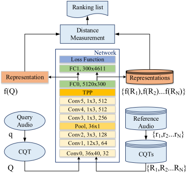
Our network consists of convolutional layers for representation learning and TPP to convert inputs into fixeddimensional vectors. When training, we consider different renditions of the same composition as samples belonging to the same category, and consider different songs as different classes. Gathering 100K recordings, we train the network through classification criteria. After the training, the output of the last but one layer is used to extract music representations as shown in Figure 1. In the retrieval process, we extract music representation of a query q through the network and used to compute the distances to music representations of the references {r1, r2 . . . rN} in the dataset. Music representations of the references are pre-computed and stored in disks for retrieval.
3.1 Low-level Representation
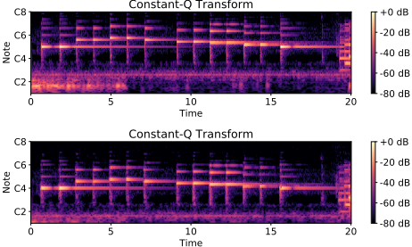
CQT is a transform with logarithmic frequency scale, reflecting western musical scale [Brown, 1991]. We use Librosa for extraction [McFee et al., 2015]. The audio is resampled to 22050 Hz. Hann window is used in preprocessing with a hop size of 512. Finally, CQT is downsampled with an averaging factor of 20. Two examples of CQTs are visualized in Figure 2, where the x-axis and y-axis represent time and frequency dimension respectively. The segments displayed in the figure represent the notes and their harmonic series in music. Compared to Chroma widely used in CSI systems [Ellis and Poliner, 2007; Serr`a et al., 2008], CQT is a low-level descriptor as it does not map frequency components into pitch classes. It remains more information and helps neural networks to learn a better representation for CSI.
3.2 Convolutional Neural Network for Key-invariance
Key transposition refers to that a piece is transposed to a different key. Figure 2 shows an example of key transposition. One could learn that if moving the notes of one figure vertically, we obtain another figure. However, matching the two figures directly (without consideration of transposition) results in high discrepancy. To deal with key transposition, some researchers tested all or some potential transpositions [Bello, 2007; Serr`a et al., 2009]. Others attempted to extract a feature invariant to key transposition [Bertin-Mahieux and Ellis, 2012; Seetharaman and Rafii, 2017].
However, these methods involve complicated hand-crafted features for key transposition. Alternatively, CNN is used to learn key-invariant representation in our approach. Viewing CQTs as images, we find that key-invariant representation is related to shift-invariant representation in image classification. Instead of recognizing objects in images, CNN is used to capture chord patterns or melodic structures frommusic. [Xu et al., 2018] used CNN to learn a key-invariant representation too but their solution used Chroma and aimed at learning a recurrent-invariant feature. Our approach is straight-forward but effective; we learn a shift-invariant feature using CNN and obtain higher precision (see Section 5.3).
The network structure is shown in Figure 1. We design Conv0 with a size of 36 × 40. This design has two advantages. First, its height is a multiple of 12. In other words, it captures four harmonics and spans three octaves. Second, to aggregate information within large contexts, its width is set as 40, corresponding to 20 s. The design is consistent with the ideas of existing works in CSI [Serr`a et al., 2008; Bertin-Mahieux and Ellis, 2012]; they usually extracted features or measured the similarity from a long range.
Obviously, the network structure is different from that in image classification or image retrieval, which consists of small square filters [Simonyan and Zisserman, 2015; He et al., 2016]. We build networks with small filters following Fully-connected layers this style initially but get poorer results. Looking into the difference between image and music, we realize that music is inherently temporal signals; even though Figure 2 shows the CQTs as images, the x-axis and y-axis have different meanings, representing time and frequency domain respectively. Hence borrowing the network structure from image classification is not appropriate. Alternatively, we utilize large kernels in the initial layers, which return better results in the experiments.
3.3 Temporal Pyramid Pooling
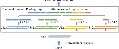
Utilizing several convolutional and pooling layers, we acquire a feature map with a shape of L × 512 in Conv5 (see Figure 1). L depends on the length of input rather than a constant; we get variable-length activations related to the inputs in this layer. Motivated by Pyramid Pooling in computer vision [He et al., 2015; Wang et al., 2017], we use TPP to learn a fixed-dimensional feature and extract information from different temporal scales. In our implementation, adaptive windows are used for pooling operations. For a pyramid level with n bins, a max-pooling window moves across the feature map through time, where i-th bin is related to the feature map within [⌊ i-1 n L⌋, ⌈ in L⌉). As shown in Figure 3, four pyramid levels {1, 2, 3, 4} are used in our approach. After this operation, we concatenate the feature maps from different levels and obtain a fixed-dimensional vector for further process.
TPP converts a variable-length feature into a fixed-length output. Without TPP, neural networks require fixed-length inputs, which are not cases of music. Another solution to tackle the difficulty of variable-length inputs may be scaling music signal into a constant length. However, audio is different from images, which can be resized into any arbitrary sizes. Although researchers proposed time stretching to scale audio, these algorithms introduced artificial effects to the original signals [Z¨olzer, 2011]. Instead of modifying signals, we leverage TPP to solve this conflict and learn fixeddimensional representations from songs with different duration.
Adopting TPP helps aggregate information from different temporal scales. It captures chord patterns and melodic structures within different parts of music. Adaptive global pooling is a particular case of TPP which employs only one pyramid level. Compared to adaptive global pooling, multiple pyramid pooling keeps more information, and we find that several pooling levels help improve precision in the experiment.
3.4 Multi-length Training
TPP is applied to transform variable-length features into fixed-dimensional vectors, which are then fed into two fully-connected layers. We are given a training set D = {(x1, t1), (x2, t2) . . . (xN, tN)} where xn represents a music version, and tn is an one-hot encoding vector, indicating to which song xn belongs. Each song has various music versions. The songs are viewed as classes, and different versions of the same song are seen as the samples from the same class. When training, we first extract CQTs {X1,X2 . . .XN} from {x1, x2 . . . xN} and feed them into the network. The network is trained using cross-entropy loss to predict the label {t1, t2 . . . tN}. However, for retrieval or testing, the network is not used to predict the category of input audio. Instead, as shown in Figure 1, we use the feature map of the last but one layer for retrieval.
Different songs have different duration. To train a model robust against duration changes, we devise a multi-length training strategy. In each training step, we sample a batch of data B ⊂ D and extract CQTs. For each CQT, we randomly crop three subsequences with a length of 200, 300 and 400, corresponding to 100 s, 150 s and 200 s respectively. If the original length is smaller 200, 300 or 400, zero elements are padded into the end of CQT sequence. Therefore, we generate three new batches B200, B300 and B400 from B, which are fed into the network for training. The motivation behind this scheme is that if we only provide the network with fixedlength inputs, the network will be biased toward this specific length. Under the circumstance, even though TPP could convert varying-length sequences into fixed-dimensional features, TPP becomes ineffective in the training process. In addition, multi-length training strategy increases the amount of training data by three times, and cropping the sequences randomly serves as a way for data augmentation. The training strategy simulates deletion changes, i.e. musicians skip music phrases or music sections when performing, and thus improves the robustness of model against structure variations too.
3.5 Retrieval
The retrieval process is shown in Figure 1. Given a query q, we extract the CQT descriptor Q and feed it into network to extract music representation f(Q), where f maps a CQT to a music representation through the network. For the references {r1, r2 . . . rN}, we extract the CQT descriptors {R1, R2 . . . RN} and compute the music representations {f(R1), f(R2) . . . f(RN)} in preprocessing. The distance dq,r between a query q and a reference r (the subscript is omitted for simplicity) is defined as cosine distance of their music representation as below:
For retrieval, we compute pair-wise distances between the query and references in the dataset, and return a ranking list for evaluation. It is worth noting that owing to computaion capacity of modern computer and low dimension of music representation, our approach could work fast on million song datasets without any acceleration.
4 Experimental Settings
4.1 Dataset
Second Hand Songs 100K (SHS100K), collected by [Xu et al., 2018], includes 8858 songs with a variety of versions and 108523 recordings totally. We split it into three subsets, namely SHS100K-TRAIN, SHS100K-VAL and SHS100K-TEST, with a ratio of 8 : 1 : 1 for training, validation and testing respectively. Unlike the partition in [Xu et al., 2018], we want to gather a larger testing set. SHS100K is highly imbalanced; some songs have tens of covers while some only have one or two covers. To make the training set more balanced, only songs with more than five covers are used for training. After the screening process, 4611 songs with 84340 recordings are used for training. For testing, we compute the similarity of all pairs of recordings in SHS100KTEST, which has 10547 recordings, and thus a 10547×10546 similarity matrix is computed for evaluation.
Youtube is collected by [Silva et al., 2016]. It consists of 50 compositions with diverse music styles and genres - each with 7 versions and thus has 350 recordings in total. The data is split into a training set and a testing set originally. To allow comparison with the literature, we use the training set as reference and testing set as query following the same configuration to [Silva et al., 2016].
Covers80 has 80 songs and every song has 2 covers. It is widely used as a benchmark dataset in the literature. To compare with existing methods, we compute the similarity of all pairs of recordings and thus a 160 × 159 similarity matrix is computed for evaluation.
4.2 Evaluation
For evaluation, we calculate the common evaluation metrics mean average precision (MAP), precision at 10 (P@10) and the mean rank of the first correctly identified cover (MR1). MAP is the mean of average precision, and P@10 is the mean ratio of the same versions identified successfully in the top 10. These metrics are exactly the ones used in Mirex Audio Cover Song Identification contest 3 . Query time is also recorded for efficiency comparison.
5 Experimental Results and Analysis
In the following experiments, we train models on SHS100KTRAIN and tune the parameters on SHS100K-VAL to select the best model. Then we evaluate the performance on the three datasets Youtube, Covers 80 and SHS100K-TEST. The proposed method is denoted as CQT-TPPNet.
5.1 Effectiveness of TPP andMulti-length Training
To compare with our model, several networks without TPP are built. Different from CQT-TPPNet, the outputs of Conv5
3 https://www.music-ir.org/mirex/wiki/2018:Audio Cover Song Identification
| MAP | P@10 | MR1 | MAP | P@10 | MR1 | MAP | P@10 | MR1 | |
|---|---|---|---|---|---|---|---|---|---|
| Results on Youtube | Results on Covers80 | Results on SHS100K-TEST | |||||||
| CQT-TPPNet | 0.859 | 0.188 | 2.85 | 0.744 | 0.086 | 6.88 | 0.465 | 0.357 | 72.2 |
| CQT-Net (200) | 0.750 | 0.174 | 3.37 | 0.618 | 0.079 | 14.7 | 0.375 | 0.305 | 109 |
| CQT-Net (300) | 0.777 | 0.176 | 3.22 | 0.681 | 0.084 | 11.5 | 0.370 | 0.305 | 104 |
| CQT-Net (400) | 0.740 | 0.179 | 3.65 | 0.636 | 0.080 | 9.48 | 0.327 | 0.277 | 107 |
| CQT-TPPNet {1, 2, 3} | 0.846 | 0.185 | 2.97 | 0.742 | 0.085 | 8.78 | 0.476 | 0.365 | 77.6 |
| CQT-TPPNet {1, 2} | 0.832 | 0.184 | 3.21 | 0.723 | 0.082 | 9.63 | 0.472 | 0.361 | 75.5 |
| CQT-TPPNet {1} | 0.828 | 0.185 | 3.62 | 0.738 | 0.082 | 8.49 | 0.430 | 0.337 | 84.1 |
| Single-length Training (200) | 0.812 | 0.180 | 3.83 | 0.722 | 0.084 | 7.14 | 0.450 | 0.348 | 86.8 |
| Single-length Training (300) | 0.815 | 0.181 | 3.41 | 0.713 | 0.082 | 7.43 | 0.422 | 0.333 | 88.9 |
| Single-length Training (400) | 0.770 | 0.175 | 4.33 | 0.658 | 0.083 | 10.3 | 0.348 | 0.291 | 108 |
| +4 semitones | 0.852 | 0.185 | 3.33 | 0.733 | 0.086 | 7.18 | 0.444 | 0.344 | 77.3 |
| -4 semitones | 0.852 | 0.186 | 3.00 | 0.724 | 0.086 | 7.59 | 0.442 | 0.344 | 78.4 |
| +12 semitones | 0.795 | 0.180 | 3.72 | 0.642 | 0.084 | 8.12 | 0.330 | 0.271 | 115 |
| -12 semitones | 0.828 | 0.185 | 3.07 | 0.709 | 0.086 | 8.14 | 0.385 | 0.309 | 91.8 |
| 0.8 × tempo | 0.824 | 0.180 | 3.44 | 0.680 | 0.085 | 9.28 | 0.385 | 0.309 | 85.2 |
| 0.9 × tempo | 0.852 | 0.186 | 3.00 | 0.728 | 0.086 | 8.18 | 0.433 | 0.339 | 79.3 |
| 1.1 × tempo | 0.828 | 0.186 | 2.86 | 0.702 | 0.083 | 7.17 | 0.425 | 0.333 | 79.4 |
| 1.2 × tempo | 0.819 | 0.183 | 3.36 | 0.674 | 0.082 | 7.89 | 0.389 | 0.311 | 86.7 |
in these networks are connected to fully-connected layers directly. These networks require fixed-length inputs for training and testing without the support of TPP. They are denoted as CQT-Net (i) where i represents the length of input, and we test i through {200, 300, 400}. Table 1 shows that TPP results in improvement. As different songs have different duration, fixing the length of input causes information loss. On the contrary, TPP is adaptive to the input and has better performance. Additionally, we explore how many pyramid levels are needed to achieve better precision. Several combinations are experimented in Table 1. Experimental results show that using several pyramid levels achieve consitently better performance than one level (or adaptive global pooling) since several levels could exploit more information from different scales. We also explore more levels than the ones shown in Table 1 but do not find notable gains. Therefore we use CQTTPPNet with four levels {1, 2, 3, 4} for the following experiments.
Several experiments are conducted to explore whether multi-length training strategy helps improve accuracy. Compared to the original setting, we train the models fixing the length of input j to {200, 300, 400} respectively, denoted as Single-length Training (j). As shown in Table 1, multi-length training achieves better performance consistently on all three datasets compared with single-length training. Multi-length training reduces the model's bias toward specific input length. Even though the models allow variable-length songs for testing, its performance degrades without using this training strategy. Another explanation of the improvement is that multi-length training provides more data for training. It is important to mention that our training set SHS100K-TRAIN has about 15 versions per song on average. Cropping segmentations randomly and feeding the networks with variable-length sequences serve as a way for data augmentation, highly boosting the performance.
5.2 Robustness against Musical Variations
Experiments have been conducted to explore the robustness of our approach against musical variations, such as key transposition and tempo change. Considering the datasets do not provide any annotation about these variations, we simulate the changes and modify the queries using Librosa [McFee et al., 2015], and then retrieve covers from the datasets and assess the performance. Since in real life musicians would not make significant changes, such as playing several octaves higher or changing tempo drastically when performing a composition, we test transpositions within one octave (or twelve semitones) and several tempo changes.
Some results are shown in Table 1, revealing that the changes result in a bit poorer performances on the datasets. Our proposed model is still able to deal with key transposition and tempo change. For instance, if the key is transposed within four semitones or tempo is changed by a factor within [0.9, 1.1], the degradation is relatively small. For key transposition, it is found that raising an octave (+12 semitones) leads to worse precision than lowering an octave (-12 semitones). Comparing the modified query with an octave either higher or lower, we find that moving up an octave by Librosa brings more artificial effects like jarring sounds than lowering an octave. These impacts make it more difficult to recognize the covers.
5.3 Comparison
We carefully reimplement two methods 2DFM [BertinMahieux and Ellis, 2012] and In-Net [Xu et al., 2018] for comparison. 2DFM is a hand-crafted feature, and In-Net utilizes neural networks for feature learning similar to our approach. The two methods and our approach are implemented on a Linux server with an Intel Xeon E5-2640v3 and two TITAN X (Pascal) GPUs. In addition, we compare with stateof-the-art methods, which report their results on Covers80 or Youtube.
| MAP | P@10 | MR1 | Time | |
|---|---|---|---|---|
| Results on Youtube | ||||
| DPLA [Serr`a et al., 2008] | 0.525 | 0.132 | 9.43 | 2420s |
| SiMPle [Silva et al., 2016] | 0.591 | 0.140 | 7.91 | 18.7s |
| Fingerprinting [Seetharaman and Rafii, 2017] | 0.648 | 0.145 | 8.27 | - |
| SuCo-DTW [Silva et al., 2018] | 0.800 | 0.180 | 3.42 | 4.59s |
| 2DFM [Bertin-Mahieux and Ellis, 2012] | 0.448 | 0.117 | 12.2 | 0.08ms |
| In-Net [Xu et al., 2018] | 0.656 | 0.155 | 6.26 | 0.05ms |
| CQT-TPPNet | 0.859 | 0.188 | 2.85 | 0.04ms |
| Results on Covers80 | ||||
| NCP-WIDI [Cheng et al., 2017] | 0.645 | - | - | - |
| CRP [Serr`a et al., 2009] | 0.544 | 0.061 | - | - |
| Fusing [Chen et al., 2018] | 0.625 | 0.071 | - | - |
| 2DFM [Bertin-Mahieux and Ellis, 2012] | 0.381 | 0.053 | 33.6 | 0.13ms |
| In-Net [Xu et al., 2018] | 0.506 | 0.068 | 16.4 | 0.07ms |
| CQT-TPPNet | 0.744 | 0.086 | 6.88 | 0.06ms |
| Results on SHS100K-TEST | ||||
| 2DFM [Bertin-Mahieux and Ellis, 2012] | 0.104 | 0.113 | 415 | 12.6ms |
| In-Net [Xu et al., 2018] | 0.219 | 0.204 | 174 | 4.53ms |
| CQT-TPPNet | 0.465 | 0.357 | 72.2 | 3.68ms |
The comparison results are shown in Table 2. It can be seen that our approach performs better than those methods on Covers80 and Youtube with respect to precision and efficiency. For example, it obtains a MAP of 0.744 and processes a query within 0.06 ms on average on Covers80. As these results were reported from different machines and operating systems except our implemented methods, query time is provided as a reference only rather than a precise comparison. Nevertheless, apart from 2DFM, In-Net and CQT-TPPNet, the methods involve sequence alignment process, requiring quadratic time complexity, and essentially run slower than our approach. Compared to 2DFM and In-Net, our approach learns a lower dimensional representation and works slightly faster. With linear time complexity, the average query time of our approach is proportional to the scale of dataset. Our approach is estimated to process a query within 1 s even for a million song dataset.
For SHS100K-TEST, our approach also obtains the highest precision with low time complexity compared to our implemented methods. Comparing the performance among different datasets, we find accuracy degrades on a larger dataset. It is because that a larger dataset is more likely to have songs sharing similar melodic structure, chord pattern and accompaniment, making it challenging to identify covers. Researchers found similar results; for example [Bertin-Mahieux and Ellis, 2012] obtained a MAP of 0.09475 on a music collection with 12960 recordings.
5.4 Error Analysis
Finally, we investigate the performance of our approach on different types of music on Covers80. Considering Covers80 has no annotation about style, we listen to the recordings carefully and given a piece of music, we annotate whether it is rock music, whether its tempo is fast and whether it has a notable accompaniment.
Then we count the error cases within different kinds. Table 3 shows that when the query is rock music or presents notable accompaniments, the error rate is relatively high. In contrast, if the accompaniment is weak and it is not rock music, the model performs better and error rate decreases to 0.39 and 0.27 respectively. We reason that rock music has more drums and cymbals, and strong accompaniment contains nonharmonic contents, making it difficult to identify the covers. How to extract representations robust against these effects is an important topic for our future work.
| Number | Error cases | Error rate | |
|---|---|---|---|
| Rock | 47 | 23 | 0.49 |
| Non-rock | 113 | 44 | 0.39 |
| Fast tempo | 90 | 36 | 0.40 |
| Slow tempo | 70 | 31 | 0.44 |
| Strong accompaniment | 115 | 55 | 0.48 |
| Weak accompaniment | 45 | 12 | 0.27 |
Furthermore, we listen to the top 10 candidates of some queries on the three datasets. Our model is able to discover cover versions including non-lyrical versions, accompaniment-only versions, versions performed in different instruments, etc. Additionally, we find that the top 10 candidates often have similar melodic structure, chord pattern and genre to the queries, though some of the candidates are not the covers of the query. For example, when the query song is rock music, the model might wrongly retrieve several rock songs as the top 10 candidates but they are not the covers of the query 4 . We reason that using music similarity as a training objective, the model learns to retrieve music sharing similar styles, not just music covers. In some sense, our model could be used for content-based music recommendation.
6 Conclusion
In this paper, we have proposed a CNN structure with Temporal Pyramid Pooling for cover song identification. It allows variable-length songs as framework input and extracts a robust representation for cover song retrieval. In addition, a training scheme is designed for network training. Extensive experiments show that our approach is robust against musical variations in covers like key transposition and tempo changes. It outperforms state-of-the-art methods on two public datasets Youtube and Covers80, and achieves the highest precision on SHS100K-TEST compared to our implemented methods with low time complexity.
@inproceedings{ijcai2019p673,
  title     = {Temporal Pyramid Pooling Convolutional Neural Network for Cover Song Identification},
  author    = {Yu, Zhesong and Xu, Xiaoshuo and Chen, Xiaoou and Yang, Deshun},
  booktitle = {Proceedings of the Twenty-Eighth International Joint Conference on
               Artificial Intelligence, {IJCAI-19}},
  publisher = {International Joint Conferences on Artificial Intelligence Organization},
  editor    = {Sarit Kraus},
  pages     = {4846--4852},
  year      = {2019},
  month     = {8},
  note      = {Main track},
  doi       = {10.24963/ijcai.2019/673},
  url       = {https://doi.org/10.24963/ijcai.2019/673},
}
TY - CPAPER TI - Temporal Pyramid Pooling Convolutional Neural Network for Cover Song Identification AU - Yu, Zhesong AU - Xu, Xiaoshuo AU - Chen, Xiaoou AU - Yang, Deshun T2 - Proceedings of the Twenty-Eighth International Joint Conference on Artificial Intelligence, IJCAI-19 PB - International Joint Conferences on Artificial Intelligence Organization PY - 2019 SP - 4846 EP - 4852 DO - 10.24963/ijcai.2019/673 UR - https://doi.org/10.24963/ijcai.2019/673 ER -Copied
Machine-readable versions of this paper, for tools and AI agents:





