
Efficient Non-parametric Bayesian Hawkes Processes
Proceedings of the Twenty-Eighth International Joint Conference on Artificial Intelligence. Main track. Pages 4299-4305.
https://doi.org/10.24963/ijcai.2019/597
Keywords
- Machine Learning: Time-series;Data Streams
- Machine Learning: Learning Generative Models
- Machine Learning: Probabilistic Machine Learning
Abstract
In this paper, we develop an efficient non-parametric Bayesian estimation of the kernel function of Hawkes processes. The non-parametric Bayesian approach is important because it provides flexible Hawkes kernels and quantifies their uncertainty. Our method is based on the cluster representation of Hawkes processes. Utilizing the stationarity of the Hawkes process, we efficiently sample random branching structures and thus, we split the Hawkes process into clusters of Poisson processes. We derive two algorithms --- a block Gibbs sampler and a maximum a posteriori estimator based on expectation maximization --- and we show that our methods have a linear time complexity, both theoretically and empirically. On synthetic data, we show our methods to be able to infer flexible Hawkes triggering kernels. On two large-scale Twitter diffusion datasets, we show that our methods outperform the current state-of-the-art in goodness-of-fit and that the time complexity is linear in the size of the dataset. We also observe that on diffusions related to online videos, the learned kernels reflect the perceived longevity for different content types such as music or pets videos.
- [Adams et al., 2009] Ryan Prescott Adams, Iain Murray, and David J C MacKay. Tractable nonparametric bayesian in- ference in poisson processes with gaussian process inten- sities. pages 9-16, 2009.
- [Bacry and Muzy, 2014] Emmanuel Bacry and Jean- Francois Muzy. Second order statistics characterization of hawkes processes and non-parametric estimation. arXiv preprint, 2014.
- [Bacry et al., 2017] Emmanuel Bacry, Martin Bompaire, Stéphane Gaïffas, and Soren Poulsen. tick: a python li- brary for statistical learning, with a particular emphasis on time-dependent modeling. ArXiv preprint, 2017.
- [Celeux and Diebolt, 1985] Gilles Celeux and Jean Diebolt. The sem algorithm: A probabilistic teacher algorithm de- rived from the EM algorithm for the mixture problem. Comp. Stat. Quarterly, 2:73-82, 1985.
- [Dempster et al., 1977] Arthur P Dempster, Nan M Laird, and Donald B Rubin. Maximum likelihood from incom- plete data via the em algorithm. Journal of the Royal Sta- tistical Society, Series B, 39(1):1-38, 1977.
- [Diggle et al., 2013] Peter J Diggle, Paula Moraga, Barry Rowlingson, and Benjamin M Taylor. Spatial and spatio- temporal log-gaussian cox processes: extending the geo- statistical paradigm. Statistical Science, 28(4):542-563, 2013.
- [Donnet et al., 2018] Sophie Donnet, Vincent Rivoirard, and Judith Rousseau. Nonparametric bayesian estimation of multivariate hawkes processes. arXiv preprint, 2018.
- [Flaxman et al., 2017] Seth Flaxman, Yee Whye Teh, and Dino Sejdinovic. Poisson intensity estimation with repro- ducing kernels. In AISTATS, pages 270-279, 2017.
- [Halpin, 2013] Peter F Halpin. A scalable em algorithm for hawkes processes. New Developments in Quantitative Psy- chology, pages 403-414, 2013.
- [Hawkes and Oakes, 1974] Alan Hawkes and David Oakes. A cluster process representation of a self-exciting process. Journal of Applied Probability, 11(3):493-503, 1974.
- [Hawkes, 1971] Alan Hawkes. Spectra of some self-exciting and mutually exciting point processes. Biometrika, 58(1):83-90, 1971.
- [Ishwaran and James, 2001] Hemant Ishwaran and Lancelot F James. Gibbs sampling methods for stick- breaking priors. Journal of the American Statistical Association, 96(453):161-173, 2001.
- [Kurashima et al., 2018] Takeshi Kurashima, Tim Althoff, and Jure Leskovec. Modeling interdependent and periodic real-world action sequences. In WWW, pages 803-812, 2018.
- [Lewis and Mohler, 2011] Erik Lewis and George Mohler. A nonparametric em algorithm for multiscale hawkes pro- cesses. Journal of Nonparametric Statistics, 1(1):1-20, 2011.
- [Linderman and Adams, 2015] Scott W Linderman and Ryan P Adams. Scalable bayesian inference for excitatory point process networks. arXiv preprint, 2015.
- [Lloyd et al., 2015] Chris Lloyd, Tom Gunter, Michael A Osborne, and Stephen J Roberts. Variational inference for gaussian process modulated poisson processes. In ICML, pages 1814-1822, 2015.
- [Mercer, 1909] James Mercer. Functions of positive and neg- ative type, and their connection with the theory of integral equations. Philosophical Transactions of the Royal Soci- ety A, 209:415-446, 1909.
- [Mishra et al., 2016] Swapnil Mishra, Marian-Andrei Ri- zoiu, and Lexing Xie. Feature driven and point process approaches for popularity prediction. CIKM, pages 1069- 1078, 2016.
- [Møller et al., 1998] Jesper Møller, Anne Randi Syversveen, and Rasmus Plenge Waagepetersen. Log gaussian cox pro- cesses. Scandinavian journal of statistics, 25(3):451-482, 1998.
- [Rasmussen and Williams, 2005] Carl Edward Rasmussen and Christopher K I Williams. Gaussian Processes for Machine Learning. The MIT Press, 2005.
- [Rasmussen, 2013] Jakob Gulddahl Rasmussen. Bayesian inference for hawkes processes. Methodology and Com- puting in Applied Probability, 15(3):623-642, 2013.
- [Rizoiu et al., 2018] Marian-Andrei Rizoiu, Swapnil Mishra, Quyu Kong, Mark Carman, and Lexing Xie. Sir- hawkes: Linking epidemic models and hawkes processes to model diffusions in finite populations. In WWW, pages 419-428, 2018.
- [Rubin, 1972] Izhak Rubin. Regular point processes and their detection. IEEE Transactions on Information The- ory, 18(5):547-557, 1972.
- [Shirai and Takahashi, 2003] Tomoyuki Shirai and Yoichiro Takahashi. Random point fields associated with certain fredholm determinants ii: Fermion shifts and their er- godic and gibbs properties. The Annals of Probability, 31(3):1533-1564, 2003.
- [Walder and Bishop, 2017] Christian J Walder and Adrian N Bishop. Fast bayesian intensity estimation for the perma- nental process. In ICML, pages 3579-3588, 2017.
- [Xu et al., 2016] Hongteng Xu, Mehrdad Farajtabar, and Hongyuan Zha. Learning granger causality for hawkes processes. In ICML, pages 1717-1726, 2016.
- [Xu et al., 2018] Hongteng Xu, Dixin Luo, Xu Chen, and Lawrence Carin. Benefits from superposed hawkes pro- cesses. AISTATS, pages 623-631, 2018.
- [Zhao et al., 2015] Qingyuan Zhao, Murat A Erdogdu, Hera Y He, Anand Rajaraman, and Jure Leskovec. Seis- mic: A self-exciting point process model for predicting tweet popularity. In SIGKDD, pages 1513-1522, 2015.
- [Zhou et al., 2013a] Ke Zhou, Hongyuan Zha, and Le Song. Learning social infectivity in sparse low-rank networks using multi-dimensional hawkes processes. In AISTATS, pages 641-649, 2013.
- [Zhou et al., 2013b] Ke Zhou, Hongyuan Zha, and Le Song. Learning triggering kernels for multi-dimensional hawkes processes. In ICML, pages III-1301-III-1309, 2013.
References were extracted automatically from the PDF and may contain errors.
Full text extracted automatically from the PDF; figures, tables and equations may differ. The PDF is the version of record.
1 Introduction
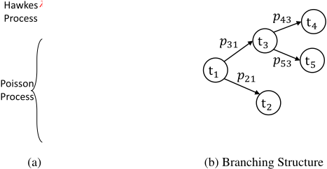
The Hawkes process [Hawkes, 1971] is a useful model of self-exciting point data in which the occurrence of a point increases the likelihood of arrival of new points. More specifically, every point causes the conditional intensity function λ - which modulates the arrival rate of new points - to increase. An alternative representation of the Hawkes process is a cluster of Poisson processes [Hawkes and Oakes, 1974], which categorizes points into immigrants and offspring. Immigrant points are generated independently at a background rate µ; offspring points are triggered by existing points at a rate of φ. Points can therefore be structured into clusters, where each cluster contains a point and the offspring it directly generated. This leads to a tree structure, also known as the branching structure (an example is shown in Fig. 1).
Background & Motivations
φ is important as it is shared and decides the class of the whole process and recently the Hawkes process with various φ has been studied. Mishra et al. [2016] employ the branching factor of the Hawkes process with the power-law kernel to predict popularity of tweets; Kurashima et al. [2018] predict human actions using a Hawkes process equipped with exponential, Weibull and Gaussian mixture kernels; online popularity unpredictability is explained using the Hawkes process with a variant of the exponential kernel by Rizoiu et al. [2018]. However, most work employes Hawkes process with parametric kernels, which encodes strong assumptions, and limits the expressivity of the model. Can we design a practical approach to learn flexible representations of the optimal Hawkes kernel function φ from data?
A typical solution is the non-parametric estimation of the kernel function [Lewis and Mohler, 2011; Zhou et al., 2013b; Bacry and Muzy, 2014].These are all frequentist methods which do not quantify the uncertainty of the learned kernels. There exists work [Rasmussen, 2013; Linderman and Adams, 2015] on the Bayesian inference for the Hawkes process. To scale past toy-dataset sizes these methods require either parametric triggering kernels or discretization of the input domain, which in turn leads to poor scaling with the dimension of the domain and sensitivity to the choice of discretization. The work closest to our own is that of Donnet et al. [2018], however their main contributions are theoretical; on the practical side they resort to an unscalable Markov chain Monte Carlo (MCMC) estimator. We comparatively summarize related works in Table 1. To the best of our knowledge, our work is the first work proposing a Bayesian nonparametric Hawkes process estimation procedure, with a linear time complexity allowing it to be applied to real-world datasets, and without requiring discretization of domains.
| Methods | Time Complexity | Bayesian | Continuous | Non-parametric |
|---|---|---|---|---|
| Zhou et al. [2013a] | O(n3 ) | � | ✓ | � |
| Xu et al. [2016] | O(n3 ) | � | ✓ | � |
| Lewis and Mohler [2011] | O(n3 ) | � | � | ✓ |
| Zhou et al. [2013b] | O(n3 ) | � | � | ✓ |
| Rasmussen [2013] | O(n) | ✓ | ✓ | � |
| Linderman and Adams [2015] | O(n) | ✓ | interval-sensored | � |
| Donnet et al. [2018] | unspecified | ✓ | ✓ | ✓ |
| Ours | O(n) | ✓ | ✓ | ✓ |
Contributions
In this paper, we propose a general framework for the efficient non-parametric Bayesian inference of Hawkes processes.
- We exploit block Gibbs sampling [Ishwaran and James, 2001] to iteratively sample the latent branching structure, the background intensity µ and the triggering kernel φ. In each iteration, the point data are decomposed as a cluster of Poisson processes based on the sampled branching structure. This is exemplified in Fig. 1, in which a Hawkes process (shown on the top temporal axis of Fig. 1a) is decomposed into several Poisson processes (the following temporal axes); the corresponding branching structure is shown in Fig. 1b. The posterior µ and φ are estimated using the resulting cluster processes. Our framework is close to the stochastic ExpectationMaximization (EM) algorithm [Celeux and Diebolt, 1985] where posterior µ and φ are estimated [Lloyd et al., 2015; Walder and Bishop, 2017] in the M-step and random samples of µ and φ are drawn. We adapt the approach of the recent non-parametric Bayesian estimation for Poisson process intensities, termed Laplace Bayesian Poisson process (LBPP) [Walder and Bishop, 2017], to estimate the posterior φ given the sampled branching structure.
- We utilize the stationarity of the Hawkes Process to speed up sampling and computing the probability of the branching structure. We theoretically show our method to be of linear time complexity. Furthermore, we explore the connection with the EM algorithm [Dempster et al., 1977] and develop a second variant of our method, as an approximate EM algorithm.
- We empirically show our method enjoys linear time complexity and can infer known analytical kernels, i.e., exponential and sinusoidal kernels. On two large-scale social media datasets, our method outperforms the current state-ofthe-art non-parametric approaches and the learned kernels re-
flect the preceived longevity for different content types.
2 Preliminaries
In this section, we introduce the prerequisites of our work: the Hawkes process and LBPP.
The Hawkes Process [Hawkes, 1971]
Introduced in Section 1, the Hawkes process can be specified using the conditional intensity function λ which modulates the arrival rate of points. Mathematically, conditioned on a set of points ttiuNi�1 , the intensity λ is expressed as:
,
where µ ¡ 0, considered as a constant, and φp�q : R � r0,8q are the background immigrant intensity and the triggering kernel. The log-likelihood of ttiuNi�1 given µ and φp�q is [Rubin, 1972]:
where Ω is the sampling domain of ttiuNi�1 .
Laplace Bayesian Poisson Process (LBPP)
LBPP [Walder and Bishop, 2017] has been proposed for the non-parametric Bayesian estimation of the intensity of a Poisson process. To satisfy non-negativity of the intensity function, LBPP models the intensity function λ as a permanental process [Shirai and Takahashi, 2003], i.e., λ � g � f where the link function gpzq � z2 {2 and fp�q obeys a Gaussian process (GP) prior. Alternative link functions include expp�q [Møller et al., 1998; Diggle et al., 2013] and gpzq � λ� p1 � expp�zqq�1 [Adams et al., 2009] where λ� is constant.
The choice gpzq � z2 {2 has the analytical advantages; for some covariances the log-likelihood can be computed in closed form [Lloyd et al., 2015; Flaxman et al., 2017]. LBPP exploits the Mercer expansion [Mercer, 1909] of the GP covariance function kpx, yq � Covpfpxq, fpyqq,
where for non-degenerate kernels, K � 8. The eigenfunctions teip�qui are chosen to be orthonormal in L2 pΩ,mq for some sample space Ω with measure m. fp�q can be represented as a linear combination of eip�q [Rasmussen and Williams, 2005], fp�q � ωT ep�q, and ω has a Gaussian prior, i.e., ω � Np0, Λq where Λ � diagpλ1, λ2, � � � , λKq is a diagonal covariance matrix and ep�q � re1p�q, � � � , eKp�qsT is a vector of basis functions. Computing the posterior distribution of the intensity function λp�q is equivalent to estimating the posterior distribution of ω which, in LBPP, is approximated by a normal distribution (a.k.a Laplace approximation [Rasmussen andWilliams, 2005]), i.e.,
where X� ttiuNi�1 is a set of point data, Ω the sample space and k the Gaussian process kernel function. ˆω is selected as the mode of the true posterior and Q the negative inverse Hessian of the true posterior at ˆw:
ω
The approximate posterior distribution of fptq is a normal distribution [Rasmussen and Williams, 2005]:
Furthermore, the posterior of λptq is a Gamma distribution:
where α � pν 2 � σ2 q2 {p4ν 2σ2 � 2σ4 q and β � pν 2 � σ2 q{p2ν 2σ2 � σ4 q.
3 Inference via Sampling
We now detail our efficient non-parametric Bayesian estimation algorithm, which samples the posterior of µ (constant background intensity) and φp�q (the trigerring kernel). Our method starts with random µ0, φ0p�q and iterates by cycling through the following four steps (k is the iteration index):
- i Calculate ppB|X, φk�1, µk�1q, the distribution of the branching structure B given the data X, triggering kernel φk�1, and background intensity µk�1 (see Section 3).
- ii Sample a Bk as per ppB|X, φk�1, µk�1q (see Section 3).
- iii Estimate ppφ|Bk,Xq (Section 3) and ppµ|Bk,Xq (Section 3).
- iv Sample a φkp�q and µk from ppφp�q|Bk,Xq and ppµ|Bk,Xq, respectively.
By standard Gibbs sampling arguments, the samples of φp�q and µ drawn in the step (iv) converge to the desired posterior, modulo the Laplace approximation in (iii). As the method is based on block Gibbs sampling [Ishwaran and James, 2001], we term it Gibbs-Hawkes.
Distribution and Sampling of the Branching Structure
The branching structure B has a data structure of tree (as Fig. 1(b)) and consists of independent triggering events. Thus, the probability of the branching structure B is the product of probabilities of triggering events, i.e., ppBq � -Ni�1 pij where pij is the probability of tj triggering ti. Given µ and φp�q, pij is the ratio between φpti �tjq and λptiq (see e.g. [Lewis and Mohler, 2011]):
Similarly, the probability of point ti being from µ, say pi0, is:
Given these probabilities we may sample a branching structure by sampling a parent for each ti according to probabilities tpijuj¥0. The sampled branching structure separates a set of points into immigrants and offspring (introduced in Section 1). Immigrants can be regarded as a sequence generated from PP(µ), where PPp�q is a Poisson process which has an intensity µ, and used to estimate the posterior µ.
The key property which we exploit in the subsequent Section 3 and Section 3 is the following. Denote by ttpiq k uNti k�1 the Nti offspring generated by point ti. If such a sequence is aligned to an origin at ti, yielding Sti � ttpiq k � tiuNi k�1 , then the aligned sequence is drawn from PP(φp�q) over [0, T-ti] where r0, Ts is the sample domain of the Hawkes process. The posterior distribution of φp�q is estimated on all such aligned sequences.
Posterior Distribution of µ
Continuing from the observations in Section 3, note that if we are given a set of points ttiuNi�1 generated by PP(µ) over Ω � r0, Ts, the likelihood for ttiuNi�1 is the Poisson likelihood, ppttiuNi�1 |µ,Ωq � e�µT pµTqN {N!. For simplicity, we place a conjugate (Gamma) prior on µT, µT � Gammapα, βq; the Gamma-Poisson conjugate family conveniently gives the posterior distribution of µT, i.e., ppµT |ttiuNi�1 , α, βq � Gammapα � N, β � 1q. We choose the scale α and the rate β in the Gamma prior by making the mean of the Gamma posterior equal to N and the variance N{2, which is easily shown to correspond to α = N and β = 1. Finally, due to conjugacy we obtain the posterior
Posterior Distribution of φp�q
We handle the posterior distribution of the triggering kernel φp�q given the branching structure in an analogous manner to the LBPP method of Walder and Bishop [2017]. That is, we assume that φp�q � f 2 p�q{2 where fp�q is Gaussian process distributed as described in Section 2. In line with [Walder and Bishop, 2017], we consider the sample domain r0, πs and the so-called cosine kernel,
,
Here, γ is a multi-index with non-negative (integral) values, r�s is the indicator function, a and b are parameters controlling the prior smoothness, and we let m � 2. This basis is orthonormal w.r.t. the Lebesgue measure on Ω � r0, πs. The expansion Eq. (12) is an explicit kernel construction based on the Mercer expansion as per Eq. (3), but other kernels may be used, for example by Nystr¨om approximation [Flaxman et al., 2017] of the Mercer decomposition.
As mentioned at the end of Section 3, by conditioning on the branching structure we may estimate φp�q by considering the aligned sequences. In particular, letting Sti denote the aligned sequence generated by ti, the joint distribution of ω and tSti ui is calculated as [Walder and Bishop, 2017]
logppω,tSti ui |Ω,kq
Note that there is a subtle but important difference between the integral term above and that of Walder and Bishop [2017], namely the limit of integration; closed-form expressions for the present case are provided in the online supplement 1 . Putting the above equation into Eq. (5) and Eq. (6), and we obtain the mean ˆω and the covariance Q of the (Laplace) approximate log-posterior in ω:
ω
Then, the posterior φ is achieved by Eqs. (7) and (8).
Computational Complexity
For LBPP, constructing Eq. (15) and Eq. (17) takes OpNoK2 q where K is the number of basis functions and No is the number of offspring. Optimizing ω (Eq. (16)) is a concave problem, which can be solved efficiently. If L-BFGS is used, OpCKq will be taken to calculate the gradient on each ω where C is the number of steps stored in memory. Computing Q requires inverting a K � K matrix, which is OpK3 q. As a result, the complexity of estimating φ|B is OppNo �KqK2 q. In terms of estimating µ|B taking Op1q, the complexity of estimating µ, φ|B is linear to the number of data. While the naive complexity for pij is OpN 2 q, Halpin [2013] provides an optimized approach to reduce it to OpNq, which relies on the stationary of Hawkes processes. In the step of sampling branching structures, points with negligible impacts on another point are not sampled as its parents. Interestingly, in comparison with LBPP, while our model is in some sense more complex, it enjoys a more favorable computational complexity. In summary, we have the following complexities per iteration and in Section 5, we validate the complexity on both synthetic and real data.
4 Maximum-A-Posterior Estimation
We explore a connection between the sampler of section 3 and the EM algorithm, which allows us to introduce an analagous approximate maximumum a posteriori (M.A.P.) scheme.
| Operation | Complexity |
|---|---|
| µ|B pij φ|B overall | Op1q OpN q OppNo �KqK2 q OppN �KqK2 q |
Relationship to EM
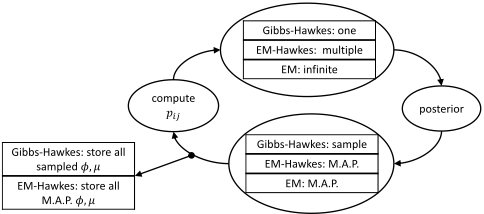
In Section 1 we mentioned the connection between our method and the stochastic EM algorithm [Celeux and Diebolt, 1985]. The difference is in the M-step; to perform EM [Dempster et al., 1977] we need only modify our sampler by: (a) sampling infinite branching structures at each iteration, and (b) re-calculating the probability of the branching structure with the M.A.P. µ and φp�q, given the infinite set of branching structures. More specifically, maximizing the expected log posterior distribution to estimate M.A.P. µ and φp�q given infinite branching structures is equivalent to maximizing the EM objective in the M-step (see the online supplement 1 for the formal derivation). Finally, note that the above step (b) is identical to the E-step of the EM algorithm.
EM-Hawkes
Following the discussion above, we propose EM-Hawkes, an approximate EM algorithm variant of Gibbs-Hawkes proposed in Section 3. Specifically, at each iteration EM-Hawkes (a) samples a finite number of cluster assignments (to approximate the expected log posterior distribution), and (b) finds the M.A.P. triggering kernels and background intensities rather than sampling them as per block Gibbs sampling (the M-step of the EM algorithm). An overview of the Gibbs-Hawkes, EM-Hawkes and EM algorithm is illustrated in Fig. 2.
Note that under our LBPP-like posterior, finding the most likely triggering kernel φp�q is intractable (see the online supplement 1 ) As an approximation we take the element-wise mode of the marginals of the φptiq to approximate the mode of the joint distribution of the φptiq.
5 Experiments
We now evaluate our proposed approaches - Gibbs-Hawkes and EM-Hawkes - and compare them to three baseline models, on synthetic data and on two large Twitter online diffusion datasets. The three baselines are: (1) A naive parametric Hawkes equipped with a constant background intensity and an exponential (Exp) triggering kernel φ � a1a2 expp�a2tq, a1, a2 ¡ 0, estimated by maximum likelihood. (2) Ordinary differential equation (ODE)-based non-parametric nonbayesian Hawkes [Zhou et al., 2013b]. (3) Wiener-Hopf (WH) equation based non-parametric non-bayesian Hawkes [Bacry and Muzy, 2014]. Codes of ODE based and WH based methods are publicly available [Bacry et al., 2017].
1 https://bit.ly/2JM6ge9
5.1 Synthetic Data
We employ two toy Hawkes processes to generate data, both having the same background intensity µ � 10, and cosine (Eq. (18)) and exponential (Eq. (19)) triggering kernels respectively:
Prediction. For three baselinemodels and EM-Hawkes, the predictions µpred and φpredp�q are taken to be the M.A.P. values, while for Gibbs-Hawkes we use the posterior mean.
Evaluation. Each toymodel generates 400 point sequences over Ω � r0, πs, which are evenly split into 40 groups, 20 for training and 20 for test. Each of the three methods fit on each group, i.e., summing log-likelihoods for 10 sequences (for the parametric Hawkes) or estimating the log posterior probability of the Hawkes process given 10 sequences (for Gibbs-Hawkes and EM-Hawkes) or fitting the superposition of 10 sequences [Xu et al., 2018]. Since the true models are known, we evaluate fitting results using the L2 distance between predicted and true µ and φp�q: dL2pgpred, gtrueq �
| Data | Exp | ODE | WH | Gibbs | EM |
|---|---|---|---|---|---|
| φcos | 0.809 | 0.677 | 1.225 | 0.414 | 0.390 |
| µcos | 1.229 | 1.262 | 30.826 | 1.381 | 2.109 |
| φexp | 0.189 | 0.965 | 1.581 | 0.235 | 0.221 |
| µexp | 1.516 | 5.471 | 82.078 | 1.818 | 3.617 |
| activeYT | 2.369 | 2.370 | 1.315 | 2.580 | 2.592 |
| SEISMIC | 3.335 | 3.357 | 2.131 | 3.576 | 3.578 |
Table 3: Empirical performance comparison between algorithms (columns) with different measures (rows). Top: L2 distance to known φ and µ, bottom: mean predictive log likelihood on real data.
Experimental Details. For Gibbs-Hawkes and EMHawkes, we must select parameters of the GP kernel (Eqs. (12) to (14)). Having many basis functions leads to a high fitting accuracy, but low speed. We found that using 32 basis functions provides a suitable balance. For kernel parameters a, b of Eq. (13), we choose a, b � 0.002. 5000 iterations are run to fit each group and first 1000 are ignored (i.e. burned-in).
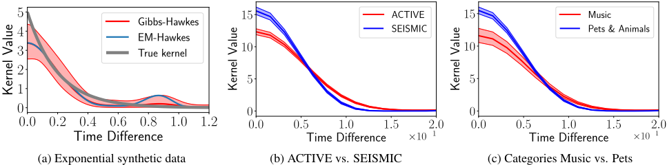
Results. The top of Table 3 shows themean L2 distance between the learned and the true φp�q and µ on toy data. GibbsHawkes and EM-Hawkes get closest triggering kernels to φcos; naturally, the parametric Hawkes - which uses an exponential kernel - fits φexp best. The parametric model retrieves µ slightly better on both synthetic datasets. The learned triggering kernels for φexp and φcos are shown in Fig. 5a and in the online supplement 1 . The ODE-based method performs well on pµcos, φcosq but badly on pµexp, φexpq. Notably, tuning the hyper-parameters of the WH method is challenging, and Table 3 shows the best result obtained after a rather exhaustive experimentation. In summary, compared with state-ofthe-art methods, our approaches achieve better performances for data generated by kernels from several parametric classes; as expected the parametric models are only effective for data generated from their own class.
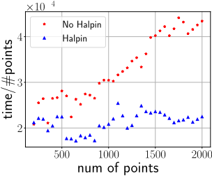
Effect of Halpin's Procedure. In Section 3 we show that using Halpin's procedure reduces the complexity of calculating pij from quadratic to linear. We now empirically validate this speed up. To distinguish between quadratic and linear complexity, we compute the ratio between running time and data size, as shown in Fig. 3. The ratio when using Halpin's procedure remains roughly constant as data size increases (the ratio increases linearly without the optimization), which implies that Halpin's procedure renders linear calculation of pij and of branching structures. Later, we will show the linear complexity of our method on real data.
5.2 Twitter Diffusion Data
We evaluate the performance of our two proposed approaches (Gibbs-Hawkes and EM-Hawkes) on two Twitter datasets, containing retweet cascades. A retweet cascade contains an original tweet, together with its direct and indirect retweets. Current state of the art diffusion modeling approaches [Zhao et al., 2015; Mishra et al., 2016; Rizoiu et al., 2018] are based on the self-exciting assumption: users get in contact with online content, and then diffuse it to their friends, therefore generating a cascading effect. The two datasets we use have been employed in prior work and they are publicly available:
- ACTIVE [Rizoiu et al., 2018] contains 41k retweet cascades, each containing at least 20 (re)tweets with links to Youtube videos. It was collected in 2014 and each Youtube video (and therefore each cascade) is associated with a Youtube category, e.g., Music or News.
- SEISMIC [Zhao et al., 2015] contains 166k randomly sampled retweet cascades, collected in from Oct 7 to Nov 7, 2011. Each cascade contains at least 50 tweets.
Setup. The temporal extent of each cascade is scaled to r0, πs, and assigned to either training or test data with equal probability. We bundle together groups of 30 cascades of similar size, and we estimate one Hawkes process for each bundle. Unlike for the synthetic dataset, for the retweet cascades dataset there is no true Hawkes process to evaluate against. Instead, we measure using log-likelihood how well the learned model generalizes to the test set. We use the same hyper-parameters values as for the synthetic data.
Fitting Performance. For each dataset, we calculate the log-likelihood per event for each tweet cascade obtained by three baselines and our approaches (Table 3). Visibly, our proposed methods consistantly outperform baselines, with EM-Hawkes performing slightly better than Gibbs-Hawkes (by 0.6% for ACTIVE and 0.4% for SEISMIC). This seems to indicate that online diffusion is influenced by factors not captured by the parametric kernel, therefore justifying the need to learn the Hawkes kernels non-parametrically. As mentioned in the synthetic data part, the WH-based method has a disadvantage of hard-to-tune hyper-parameters, which leads to the worst performance among all methods.
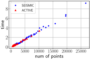
Scalability. To validate the linear complexity of our method, we record running time per iteration of GibbsHawkes on ACTIVE and SEISMIC in Fig. 4. The running time rises linearly with the number of points increasing, in line with the theoretical analysis. Linear complexity makes our method scalable and applicable on large datasets.
Interpretation. We show in Fig. 5a the learned kernels for information diffusions. We notice that the learned kernels appear to be decaying and long-tailed, in accordance with the prior literature. Fig. 5b shows that the kernel learned on SEISMIC is decaying faster than the kernel learned on ACTIVE. This indicates that non-specific (i.e. random) cascades have a faster decay than video-related cascades, presumably due to the fact that Youtube videos stay longer in the human attention. This connection between the type of content and the speed of the decay seems further confirmed in Fig. 5c, where we show the learned kernels for two categories in ACTIVE: Music and Pets & Animals. Cascades relating to Pets & Animals have a faster decaying kernel than Music, most likely because Music is an ever-green content.
6 Conclusions
In this paper, we provided the first non-parametric Bayesian inference procedure for the Hawkes process which requires no discretization of the input domain and enjoys a linear time complexity. Our method iterates between two steps. First, it samples the branching structure, effectively transforming the Hawkes process into a cluster of Poisson processes. Next, it estimates the Hawkes triggering kernel using a non-parametric Bayesian estimation of the intensity of the cluster Poisson processes. We provide both a full posterior sampler and an EM estimation algorithm based on our ideas. We demonstrated our approach can infer flexible triggering kernels on simulated data. On two large Twitter diffusion datasets, our method outperforms the state-of-the-art in held-out likelihood. Moreover, the learned non-parametric kernel reflects the intuitive longevity of different types of content. The linear complexity of our approach is corroborated on both the synthetic and real problems. The present framework is limited to the univariate unmarked Hawkes process and will be extended to marked multivariate Hawkes process.
Acknowledgements
This research was supported in part by the Australian Government through the Australian Research Council's Discovery Projects funding scheme (project DP180101985).
@inproceedings{ijcai2019p597,
  title     = {Efficient Non-parametric Bayesian Hawkes Processes},
  author    = {Zhang, Rui and Walder, Christian and Rizoiu, Marian-Andrei and Xie, Lexing},
  booktitle = {Proceedings of the Twenty-Eighth International Joint Conference on
               Artificial Intelligence, {IJCAI-19}},
  publisher = {International Joint Conferences on Artificial Intelligence Organization},
  editor    = {Sarit Kraus},
  pages     = {4299--4305},
  year      = {2019},
  month     = {8},
  note      = {Main track},
  doi       = {10.24963/ijcai.2019/597},
  url       = {https://doi.org/10.24963/ijcai.2019/597},
}
TY - CPAPER TI - Efficient Non-parametric Bayesian Hawkes Processes AU - Zhang, Rui AU - Walder, Christian AU - Rizoiu, Marian-Andrei AU - Xie, Lexing T2 - Proceedings of the Twenty-Eighth International Joint Conference on Artificial Intelligence, IJCAI-19 PB - International Joint Conferences on Artificial Intelligence Organization PY - 2019 SP - 4299 EP - 4305 DO - 10.24963/ijcai.2019/597 UR - https://doi.org/10.24963/ijcai.2019/597 ER -Copied
Machine-readable versions of this paper, for tools and AI agents:





