
Masked Graph Convolutional Network
Proceedings of the Twenty-Eighth International Joint Conference on Artificial Intelligence. Main track. Pages 4070-4077.
https://doi.org/10.24963/ijcai.2019/565
Keywords
- Machine Learning Applications: Networks
- Machine Learning: Data Mining
Abstract
Semi-supervised classification is a fundamental technology to process the structured and unstructured data in machine learning field. The traditional attribute-graph based semi-supervised classification methods propagate labels over the graph which is usually constructed from the data features, while the graph convolutional neural networks smooth the node attributes, i.e., propagate the attributes, over the real graph topology. In this paper, they are interpreted from the perspective of propagation, and accordingly categorized into symmetric and asymmetric propagation based methods. From the perspective of propagation, both the traditional and network based methods are propagating certain objects over the graph. However, different from the label propagation, the intuition ``the connected data samples tend to be similar in terms of the attributes", in attribute propagation is only partially valid. Therefore, a masked graph convolution network (Masked GCN) is proposed by only propagating a certain portion of the attributes to the neighbours according to a masking indicator, which is learned for each node by jointly considering the attribute distributions in local neighbourhoods and the impact on the classification results. Extensive experiments on transductive and inductive node classification tasks have demonstrated the superiority of the proposed method.
- [Bahdanau et al., 2015] Dzmitry Bahdanau, Kyunghyun Cho, and Yoshua Bengio. Neural machine translation by jointly learning to align and translate. In ICLR, 2015.
- [Belkin et al., 2006] Mikhail Belkin, Partha Niyogi, and Vikas Sindhwani. Manifold regularization: A geometric framework for learning from labeled and unlabeled exam- ples. JMLR, 7:2399-2434, 2006.
- [Carlson et al., 2010] Andrew Carlson, Justin Betteridge, Bryan Kisiel, Burr Settles, Estevam R. Hruschka Jr., and Tom M. Mitchell. Toward an architecture for never-ending language learning. In AAAI, pages 1306-1313, 2010.
- [Chapelle et al., 2009] Olivier Chapelle, Bernhard Scholkopf, and Alexander Zien. Semi-supervised learning (chapelle, o. et al., eds.; 2006)[book reviews]. IEEE TNN, 20(3):542-542, 2009.
- [Defferrard et al., 2016] Michaël Defferrard, Xavier Bres- son, and Pierre Vandergheynst. Convolutional neural net- works on graphs with fast localized spectral filtering. In NIPS, pages 3837-3845, 2016.
- [Duvenaud et al., 2015] David K. Duvenaud, Dougal Maclaurin, Jorge Aguilera-Iparraguirre, Rafael Gómez- Bombarelli, Timothy Hirzel, Alán Aspuru-Guzik, and Ryan P. Adams. Convolutional networks on graphs for learning molecular fingerprints. In NIPS, pages 2224-2232, 2015.
- [Gao et al., 2018] Hongyang Gao, Zhengyang Wang, and Shuiwang Ji. Large-scale learnable graph convolutional networks. In ACM SIGKDD, pages 1416-1424, 2018.
- [Hamilton et al., 2017] William L. Hamilton, Zhitao Ying, and Jure Leskovec. Inductive representation learning on large graphs. In NIPS, pages 1025-1035, 2017.
- [Kipf and Welling, 2017] Thomas N. Kipf and Max Welling. Semi-supervised classification with graph convolutional networks. In ICLR, 2017.
- [Klicpera et al., 2019] Johannes Klicpera, Aleksandar Bo- jchevski, and Stephan Günnemann. Combining neural networks with personalized pagerank for classification on graphs. In ICLR, 2019.
- [Krizhevsky et al., 2012] Alex Krizhevsky, Ilya Sutskever, and Geoffrey E. Hinton. Imagenet classification with deep convolutional neural networks. In NIPS, pages 1106- 1114, 2012.
- [Li et al., 2018] Qimai Li, Zhichao Han, and Xiao-Ming Wu. Deeper insights into graph convolutional networks for semi-supervised learning. In AAAI, pages 3538-3545, 2018.
- [Lu and Getoor, 2003] Qing Lu and Lise Getoor. Link-based classification. In ICML, pages 496-503, 2003.
- [Monti et al., 2017] Federico Monti, Davide Boscaini, Jonathan Masci, Emanuele Rodolà, Jan Svoboda, and Michael M. Bronstein. Geometric deep learning on graphs and manifolds using mixture model cnns. In IEEE CVPR, pages 5425-5434, 2017.
- [Niepert et al., 2016] Mathias Niepert, Mohamed Ahmed, and Konstantin Kutzkov. Learning convolutional neural networks for graphs. In ICML, pages 2014-2023, 2016.
- [Perozzi et al., 2014] Bryan Perozzi, Rami Al-Rfou, and Steven Skiena. Deepwalk: online learning of social rep- resentations. In ACM SIGKDD, pages 701-710, 2014.
- [Sen et al., 2008] Prithviraj Sen, Galileo Namata, Mustafa Bilgic, Lise Getoor, Brian Gallagher, and Tina Eliassi- Rad. Collective classification in network data. AI Mag- azine, 29(3):93-106, 2008.
- [Serafino et al., 2018] Francesco Serafino, Gianvito Pio, and Michelangelo Ceci. Ensemble learning for multi-type classification in heterogeneous networks. IEEE TKDE, 30(12):2326-2339, 2018.
- [Subramanian et al., 2005] Aravind Subramanian, Pablo Tamayo, Vamsi K. Mootha, Sayan Mukherjee, Ben- jamin L. Ebert, Michael A. Gillette, Amanda Paulovich, Scott L. Pomeroy, Todd R. Golub, Eric S. Lander, and Jill P. Mesirov. Gene set enrichment analysis: A knowledge-based approach for interpreting genome-wide expression profiles. Proceedings of the National Academy of Sciences, 102(43):15545-15550, 2005.
- [Veličković et al., 2018] Petar Veličković, Guillem Cucurull, Arantxa Casanova, Adriana Romero, Pietro Liò, and Yoshua Bengio. Graph attention networks. In ICLR, 2018.
- [Weston et al., 2012] Jason Weston, Frédéric Ratle, Hossein Mobahi, and Ronan Collobert. Deep learning via semi- supervised embedding. In Neural Networks: Tricks of the Trade -Second Edition, pages 639-655. 2012.
- [Yang et al., 2016] Zhilin Yang, William W. Cohen, and Ruslan Salakhutdinov. Revisiting semi-supervised learn- ing with graph embeddings. In ICML, pages 40-48, 2016.
- [Zhou et al., 2003] Dengyong Zhou, Olivier Bousquet, Thomas Navin Lal, Jason Weston, and Bernhard Schölkopf. Learning with local and global consistency. In NIPS, pages 321-328, 2003.
- [Zhu et al., 2003] Xiaojin Zhu, Zoubin Ghahramani, and John D. Lafferty. Semi-supervised learning using gaussian fields and harmonic functions. In ICML, pages 912-919, 2003.
- [Zhu, 2006] Xiaojin Zhu. Semi-supervised learning litera- ture survey. Computer Science, University of Wisconsin- Madison, 2(3):4, 2006.
- [Zitnik and Leskovec, 2017] Marinka Zitnik and Jure Leskovec. Predicting multicellular function through multi-layer tissue networks. Bioinformatics, 33(14):i190- i198, 2017.
References were extracted automatically from the PDF and may contain errors.
Full text extracted automatically from the PDF; figures, tables and equations may differ. The PDF is the version of record.
1 Introduction
Semi-supervised classification, which leverages both the labelled and unlabelled data for prediction, is a traditional yet popular topic in machine learning for both the unstructured and structured data [Chapelle et al., 2009; Zhu, 2006]. Traditional attribute-graph based semi-supervised classification (AGSS) methods, such as label propagation (LP [Zhu et al., 2003]) and label spreading (LS [Zhou et al., 2003]), can effectively classify the unstructured data, i.e., there is no structural correlations among these data samples. On the other hand, the graph convolutional neural networks
∗Corresponding author.
(GCNNs) [Niepert et al., 2016; Duvenaud et al., 2015; Gao et al., 2018], such as graph convolutional network (GCN [Kipf and Welling, 2017]) and graph attention network (GAT [Veliˇckovi´c et al., 2018]), are recently proposed for semisupervised node classification of the structured data, i.e., there exists structural correlations among these data samples.
The traditional AGSS methods usually take all the features and labels of the data samples as input. Note that only a certain portion of the data samples possesses labels and other samples are unlabelled. Then, they propagate the given labels over the graph constructed from the input features to predict the unlabelled data samples. On the contrary, GCNNs take the real graph topologies as well as the given features and labels as input. Then, they smooth the node attributes with respect to the graph topology and predict the target nodes based on the smoothed attributes [Li et al., 2018]. Many approaches with different smoothing operators have been proposed from either the spectral or spatial perspectives [Monti et al., 2017; Defferrard et al., 2016; Hamilton et al., 2017].
In this paper, we interpret GCNNs from the perspective of propagation by analyzing three latest methods, i.e., GCN [Kipf and Welling, 2017], GAT [Veliˇckovi´c et al., 2018] and PageRank GCN (PR-GCN [Klicpera et al., 2019]). Instead of propagating the labels over the attribute-based graph in traditional attribute-graph based semi-supervised classification techniques, attributes are propagated base on real graph topologies in GCNNs.
| Category | Symmetric Propagation | Asymmetric Propagation | |||
|---|---|---|---|---|---|
| Method | GCN | PR-GCN | Label Spreding | GAT | Label Propagation |
| Objective Function L | = ∑i,j wij ∥∥∥∥ hi √di - hj √dj | ∥∥∥∥2 2 L + µ ∑i ||hi - yi||22 | ∑i,j wij ||hi - hj ||22 | ||
| Graph Laplacian | ˆL = D- 1 2 WD- 12 | L = D-W | |||
| Parameters wij | aij | exp (- ∑d (xid-xjd)2 σ2d ) | exp (bT [hi ||hj ]) for connected nodes i and j | exp (- ∑d (xid-xjd)2 σ2d ) | |
| Propagation Medium | Network topology | Attribute-based network | Attribute-enhanced network topology | Attribute-based network | |
| Propagation Object | Attributes xi | Labels yi | Attributes xi | Labels yi | |
| Analytical Solution | All nodes with same hi | (1 - α)(I - α ˆL)-1 Y | Unknown | (I - Puu)-1PulYl | |
| Iteration h(k+1) i | ∑j wij √didj h(k) j | (1 - α) ∑j wij √didj h(k) j +αyi | ∑j wij di h(k) j | ||
| Propagation Symmetry | Symmetric (wij = wji) | Asymmetric wij = bT1 hi + bT2 hj wji = bT1 hj + bT2 hi | Asymmetric wij/di ̸= wji/dj although wij = wji | ||
| Constraints | h(0) i = xi | With regularization ∑i ||hi - yi||22 | h(0) i = xi | h(k) i = yi for the labelled nodes | |
| Parameter Learning | No hyper-parameters | Tune σd = σ manually | Minimize the cross entropy of the labelled data | Minimize the entropy of the unlabelled data | |
By deep analogy, both the AGSS approaches and GCNNs can be interpreted from the perspective of propagation and classfied into two categories (as shown in Table 1):
- GCN, PR-GCN and label spreading (LS) minimize the objective functions based on symmetric normalized graph Laplacian, which results in symmetric propagations.
- GAT and label propagation (LP) minimize the objective functions based on original graph Laplacian, which results in asymmetric propagations.
This unified interpretation motivates us to consider that "Should the attributes be propagated as the labels?". In general, propagation is based on the intuition that "the connected data samples tend to be similar". Typically, this intuition is valid for the labels, i.e., the connected nodes usually possess similar labels. Therefore, labels are often propagated entirely. Unfortunately, this intuition is not necessarily correct for the attributes. Different from the labels, certain attributes should not be propagated over the network. For example, the interests of a superstar tend be propagated to his fans, i.e., the fans tend to have the same interests as their idol. On the other hand, the gender of the superstar should not be propagated to his fans, because the gender of the fans cannot be changed according to the gender of the superstar. In fact, the connected nodes only possess a certain portion of similar attributes.
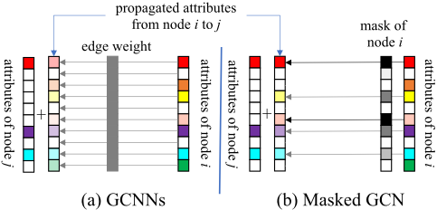
According to the observation above, a masked graph convolutional network (Masked GCN) is proposed in this paper, as described in Fig. 1. Instead of directly propagating all the attributes in each node, Masked GCN only propagates a portion of its attributes to the neighbours. The selection of the to-be-propagated attributes is achieved by assigning a mask to each node. The masks are learned by jointly considering the local and global information, i.e., the distributions of the attributes in local neighbourhoods and their impacts on the classification result. Although the backbone fully-connected network is similar to GCN, Masked GCN possesses another two interactive learnable components, the edge weights and masks for the nodes, which enhance the flexibility of our proposed Masked GCN. These three learnable components can be jointly trained by minimizing the cross-entropy between the predicted and given labels.
The contributions are summarized as follows:
- We analyze the traditional attribute-graph based semisupervised classification and graph convolutional neural networks from the perspective of propagation, and classify them into two categories, symmetric and asymmetric propagations.
- We conclude that the common assumption in label propagation cannot satisfy the practical demands of the attribute propagation and only part of the attributes should be propagated.
- We propose a masked graph convolution network (Masked GCN), which satisfies the demands of attribute propagation, by learning a mask vector for each node.
2 Notations
For a set of data samples V = {vi|i = 1, ...,N}, where |V | = N, each data sample is associated with a feature xn ∈ RT . X ∈ RN×T is the collection of these features, each row of which corresponds to a sample. If there exists a network among these data samples, it can be represented by an attributed graph G = (V, E, X), where E stands for a set of edges and each edge connects two vertices in V . The sparse adjacency matrix A = [aij ] ∈ {0, 1}N×N is employed to represent the network topology, where aij = 1 if an edge exists between the vertices vi and vj, and vice versa. If the network is allowed to possess self-edges, then ann = 1. Otherwise, ann = 0. If a network is constructed based on the node features instead of observed links, its adjacency matrix is represented as W = [wij] ∈ RN×N , which is the generalized A. dn = ∑j wnj is the degree of the vertex vn, and D = diag(d1, d2, ..., dN) is the degree matrix of the adjacency matrix W. Then, the normalized adjacency matrix is P = D-1A. The graph Laplacian and its normalized form are defined as L = D-A and ˆL = D- 12 LD- 12 , respectively.
In semi-supervised classification, the labels Yl = {yi} ∈ R|Vl|×F of a set of vertices Vl ⊂ V , where F is the number of classes, are given. For simplicity, nodes {vn}ln=1 is assumed be labelled, while nodes {vn}|V | n=l+1 are unlabelled. Then, the label matrix Yl can be reformed as Y = [Yl; Yu] ∈ R|V |×F , where Yu is a zero matrix. The normalized adjacency matrix can then be expressed as
where Pll ∈ R|Vl|×|Vl| and Puu ∈ R|V-Vl|×|V-Vl| are the sub-matrices of P which correspond to the labelled and unlabelled nodes, respectively.
3 Comparisons between AGSS and GCNNs
In this section, two traditional AGSS methods and three latest GCNNs are firstly reviewed. Then, the similarities between these two types of techniques are analyzed and summarized accordingly. Note that the symbol hi is employed to denote the object, which is propagated over the graph. Typically, the labels are the objects propagated in traditional AGSS approaches, while the attributes are the objects propagated in GCNNs. Therefore, we simply employ hi to represent both the propagated labels in AGSS classification (in Sec. 3.1), and the propagated attributes in GCNNs (in Sec. 3.2).
3.1 Traditional Attribute-graph based Semi-supervised Classification
In transductive semi-supervised learning, the unlabeled data samples given in the training stage is also the to-be-predicted data in the testing stage. Traditional AGSS approaches are well-studied transductive semi-supervised learning strategies.
A graph, which reveals the similarities between data samples, is usually constructed with edges. Let wij denote the edge between the data samples vi and vj, and it is defined as
where σd's are learnable parameters. Then, the semisupervised learning process is conducted by propagating the given labels over the constructed graph. With different propagation strategies and constraints, numerous algorithms have been proposed, such as label propagation [Zhu et al., 2003], label spreading [Zhou et al., 2003] and etc.
Label Propagation
According to Gaussian random field on the graph, where the mean of the field is characterized by the harmonic functions, Label Propagation (LP) directly minimizes the energy function
with hi = yi which is fixed as the label yi of the ith data sample in Vl. Note that H = {hi}Ni=1 is the predicted labels, L = D - A represents the graph Laplacian matrix of W and tr(.) stands for the trace operator. By minimizing Eq. (2) with respect to hi, its iterative updating formula for the unlabelled data is computed as
Then, the analytical solution can be expressed as
where I is an identity matrix with the size of |V -Vl|. The parameters σd's are learned by minimizing the average entropy of the labels for the unlabelled data, which is formulated as
with respect to σd. This strategy is based on the intuition that a well constructed graph will generate confident predictions, i.e., hi is close to either 0 or 1.
Label Spreading
By considering the smoothness property of the graph, Label Spreading (LS) formulates the propagation as H(k+1) = (1α) ˆLH(k) + αY , where ˆL is the normalized Laplacian matrix of W. This formulation is equivalent to the updating formula
which possesses the analytical solution as Eq. (7) shows.
Eq. (7) is proved to be the solution of the following objective function [Zhou et al., 2003]
with α = 1 1+µ . As can be observed, the hard constraint of the given labels in LP is replaced by a soft constraint, i.e., the regularization term ∑i ||hi - yi||22 . Here, all the hyperparameters σd's are set to be σ and tuned manually.
3.2 Graph Convolutional Neural Networks
Graph convolutional neural networks are extended from the convolutional neural network (CNN [Krizhevsky et al., 2012]) which processes structured data samples, such as images or speeches, to process the general graph data samples. Different from the traditional attribute-graph based semi-supervised learning, where only the attributes and labels are given and networks are constructed from the attributes as described in Sec. 3.1, GCNNs exploits the network topologies as well as the attributes and labels.
Graph Convolutional Network
Graph Convolutional Network (GCN) [Kipf and Welling, 2017] simplifies many previous models which possess high complexities, and defines the graph convolution operation as
with H(0) GCN = X, where ˜ A = A + IN and ˜Dnn = ∑j ˜ Anj = dn + 1. The unknown labels can be predicted by feeding H(k+1) GCN into a fully-connected layer as QGCN = HGCNW. The parameter W is obtained by minimizing the cross-entropy between the given labels and the predictions as
PageRank GCN
Since GCN is equivalent to Laplacian smoothing the attributes in the graph [Li et al., 2018], all the nodes tend to obtain identical attributes as the number of iterations (i.e. the number of graph convolutional layers) increases. To alleviate this issue, PageRank GCN (PR-GCN [Klicpera et al., 2019]) improves the original GCN by considering its relationship with PageRank. The convolution operator in PageRank GCN is defined as
Unfortunately, directly calculating the fully personalized PageRank matrix (1 - α)(I - αˆL)-1 is computationally inefficient, because it will generate a dense matrix, which will induce extra computations in the multiplication with the attribute matrix X. PR-GCN resolves this issue by approximating HPR GCN in an iterative manner as
Its prediction and training procedures are identical to GCN.
Graph Attention Network
To give consistent performances with variable sized inputs and effectively exploit the most important parts of the inputs, the attention mechanism is introduced by GAT to handle neighbourhoods with various sizes. GAT replaces the graph convolutional layer in GCN with a graph attention layer by leveraging attention mechanism [Bahdanau et al., 2015]. To obtain the nodes which should be focused on, the attention coefficients
is computed to reveal the amount of attentions received at node vk from node vn. GAT adopts the Leaky-ReLU nonlinearity mapping, LeakyReLU([xTn W||xTk W]b), as c(., .) in Eq. (13), where [xTn W||xTk W] represents the concatenation of xTn W and xTk W, and b ∈ R2F stands for the shared parameters. O = [onk] ∈ RN×N can be regarded as the re-assigned weights to the adjacency matrix A = [ank] ∈ RN×N . onk ̸= 0 when ank = 1, i.e., the nodes vn and vk are connected.
Then, GAT can be represented as QGAT = OXW and considered as a re-weighted adjacency matrix based smoothing as
with H(0) GAT = X. After the smoothing operation, a projection QGAT = HGATW is performed. The parameter W and attention parameter b can be computed by minimizing the cross-entropy between the given labels and predictions according to Eq. (10).
3.3 Comparisons
Here, the traditional AGSS techniques (in Sec. 3.1) and GCNNs (in Sec. 3.2) are analyzed from the perspective of propagation, and they are classified into two categories: symmetric and asymmetric propagations as summarized in Table 1.
Symmetric Propagation (GCN, PR-GCN and LS)
Comparing Eq. (11) and Eq. (12) with Eq. (7) and Eq. (6), respectively, the differences between PR-GCN and LS are summarized as follows: 1) the labels are propagated in LS while the attributes are propagated in PR-GCN; 2) the normalization is 1 √didj in LS and 1 √(di+1)(dj+1) in PR-GCN, because Aii = 1 in PR-GCN while Wii = 0 in LS. If self-loop is allowed in LS, its normalization will also be 1 √(di+1)(dj+1) which is identical to PR-GCN. Therefore, PR-GCN [Klicpera et al., 2019] is equivalent to LS [Zhou et al., 2003], despite the different propagated objects. The objective function of LS in Eq. (8) can also serve for PR-GCN by replacing the label yi with the attribute xi.
Comparing Eq. (12) from PR-GCN with Eq. (9) from GCN, PR-GCN averages the propagated attributes ˜D- 12 ˜ A ˜D- 1 2H and the original attributes X with weights 1 - α and α, respectively, while GCN does not perform these averages. The objective function of GCN is the first part of Eq. (8) (which is the cost function of LS), i.e., L = ∑i,j wij|| hi √di - hj √dj ||22 .
The propagation weights in GCN, PR-GCN and LS are wij √didj . Since wij = wji holds in these algorithms, their propagations are considered to be symmetric.
Asymmetric Propagation (GAT and LP)
Comparing Eq. (3) fromLPwith Eq. (14) (where onk defined in Eq. (13)) from GAT, the difference between them is the edge weight function. LP adopts Eq. (1), while GAT utilizes
if vi and vj are connected. Note that [hi||hj] is the concatenated vector of hi and hj, and hi possesses the identical size compared to hj. Therefore, their objective functions and updating formulas are the same as shown in Eqs. (2) and (3), respectively. Since wij = wji holds in LP, it performs symmetric propagations if the normalization is disabled. Since bi = bj does not exist in most of the situations, wij ̸= wji and thus LP and GAT perform asymmetric propagations.
| Dataset | #Nodes | #Edges | #Classes | #Features |
|---|---|---|---|---|
| CiteSeer | 3,327 | 4,732 | 6 | 3,703 |
| Cora | 2,708 | 5,429 | 7 | 1,433 |
| PubMed | 19,717 | 44,338 | 3 | 500 |
| NELL | 65,755 | 266,144 | 210 | 5,414 |
| PPI | 56,944 | 818,716 | 121 | 50 |
4 Masked Graph Convolutional Network
In this section, we propose our Masked Graph Convolutional Network (Masked GCN) by providing the motivations, formulations and solutions accordingly.
4.1 Motivations
With the comparisons and summaries in Sec. 3, the inherent difference between the traditional AGSS techniques and GCNNs can be considered as the object to be propagated before the predictions. Labels are propagated in traditional AGSS methods, while attributes are propagated in GCNNs. The common assumption in these methods is "the connected data samples tend to be similar". For traditional label propagations, this assumption usually holds because the connected data samples tend to possess similar labels. However, this assumption is debatable for attribute propagations. For example, each people usually has many characters in online social networks. Two connected people are often similar for some characters instead of all the characters. Therefore, the connected nodes are usually similar for a certain portion of their attributes.
4.2 Formulations and Solutions
Here, Masked Graph Convolutional Network (Masked GCN) is formulated based on asymmetric propagation and attributeenhanced network topology. According to the above intuition, the objective function is defined as follows.
where hi stands for the attributes of the node vi, and wij, which is defined in Eq. (15), represents the edge weight between the nodes vi and vj. Note that M (j) = diag(m(j) 1 ,m(j) 2 , ...,m(j) T ) is the diagonal mask matrix of the node vi, where T is the number of attributes, i.e., the length of hi (hj). This mask matrix M (j) relaxes the hard constraint that hi and hj tend to be completely similar and only constrain a certain portion of hi and hj to be similar. By minimizing Eq. (16) with respect to hi, the updating formula can be obtained ash(k+1)
As can be observed, the propagated attributes is masked by M (j) as illustrated in Fig. 1. The mask m(j) t of attribute t in node j is exploited to determine whether the attribute t in node j should be propagated to its neighbours. If m(j) t is large, most of the attribute t in node j will be propagated (e.g. the red and pink attributes in Fig. 1(b)), and vice versa (e.g. the orange and green attributes).
Then, the formulation of M (j) can be introduced. Intuitively, the mask m(j) t of the attribute t in node j should be determined by both the local and global behaviors of attribute t. Typically, m(j) t should be affected by the confidence that node i possesses attribute t. Therefore, the consistencies of attribute t between node vi and its neighbours, i.e., - ∑p∈N(j) wjp(hpt - hjt)2 , are taken in to account in the proposed method. If the consistency is low, the mask tends to prevent the attribute t from being propagated, i.e., m(j) t should be small. On the other hand, m(j) t should globally benefit the classification result. Therefore, a learnable parameter σt, which is independent of the nodes, is assigned. By jointly considering the local and global behaviors, the mask is defined as
where Σ = diag(σ1, σ2, ..., σT ) is the matrix which contains the learnable attribute weights. Similar to GCN and GAT, two backbone convolutional layers are utilized in Masked GCN, i.e., the attributes are propagated twice.
By setting H(0) Masked GCN = X which is the original attributes, H(1) Masked GCN = {h(1) i }Ni=1 and H(2) Masked GCN = {h(2) i }Ni=1 are calculated via Eq. (17). The unknown labels are predicted by feeding the obtained attributes H(2) Masked GCN into a fully-connected layer as follow.
where W is the weights in the fully-connected layer.
There exists three learnable components in the proposed Masked GCN, W in the fully-connected layer (Eq. (19)), b in edge re-weighting (Eq. (15)) and Σ = diag(σ1, σ2, ..., σT ) in the learned mask (Eq. (18)). They can be jointly trained via gradient back-propagation.
Remark 1: In GCN, all the attributes are propagated, which tend to amend all the nodes to possess the identical attributes after convergence. Since Masked GCN only propagates part of the attributes, this issue can be alleviated.
Remark 2: The formulation of Masked GCN are constructed for the transductive semi-supervised node classification task. Since GCNNs propagate attributes based on the network topology instead of propagating labels, the proposed Masked GCN can be directly applied to inductive semi-supervised node classification task where the target graphs in the testing stage are not provided in the training stage.
Remark 3: Although only GAT in asymmetric propagation is improved to the masked version, other GCNNs, such as GCN and PR-GCN in symmetric propagation, can also be improved with the proposed mask. For example, GCN can be improved to
where wij = aij is obtained from graph topology and it is not learnable as in GCN. Similar to Eq. (16), M (j) also serves as masks in Eq. (20).
| Methods | Cora | Citeseer | Pubmed | NELL |
|---|---|---|---|---|
| MLP | 55.1% | 46.5% | 71.4% | 22.9% |
| ManiReg [Belkin et al., 2006] | 59.5% | 60.1% | 70.7% | 21.8% |
| SemiEmb [Weston et al., 2012] | 59.0% | 59.6% | 71.7% | 26.7% |
| LP [Zhu et al., 2003] | 68.0% | 45.3% | 63.0% | 26.5% |
| DeepWalk [Perozzi et al., 2014] | 67.2% | 43.2% | 65.3% | 58.1% |
| ICA [Lu and Getoor, 2003] | 75.1% | 69.1% | 73.9% | 23.2% |
| Planetoid [Yang et al., 2016] | 75.7% | 64.7% | 77.2% | 61.9% |
| Chebyshev [Defferrard et al., 2016] | 81.2% | 69.8% | 74.4% | - |
| MoNet [Monti et al., 2017] | 81.7% | 69.9% | 78.8% | 64.2% |
| Random-scheme Mask GCN | 14.8% | 17.2% | 35.1% | 4.8% |
| GCN [Kipf and Welling, 2017] | 81.5% | 70.3% | 79.0% | 66.0% |
| Masked GCN (Sym) | 82.7% | 72.0% | 79.3% | 68.2% |
| GAT [Veliˇckovi´c et al., 2018] | 83.0% | 72.5% | 79.0% | - |
| Masked GCN (Asym) | 84.4% | 73.8% | 80.2% | 68.9% |
nodes and 1000 nodes are employed for training, validation and performance assessment, respectively. Besides, another bipartite large network [Carlson et al., 2010], NELL, is constructed from a knowledge graph as shown in Table 2. Except for the entity nodes in the original knowledge graph, separate relation nodes (ei, r) and (ej, r) are extracted from each entity pair (ei, r, ej). The edges are constructed between each entity ei and its all relation nodes (ei, r).
Remark 4: Although T additional learnable parameters σt's are introduced in Masked GCN, the number of additional parameters is relatively small compared to the numbers of parameters in GCN and GAT. The parameters in the one-layered GCN are the weights of the fully connected layer, whose number is T × C (where T and C are the numbers of attributes and classes, respectively). In addition to the weights of the fully connected layer, GAT also possesses another 2T parameters, which is employed to determine the weights of the edges. Therefore, the T additional learnable parameters in Masked GCN tend not to cause overfitting.
5 Evaluations
In this section, we validate the proposed Masked GCN by empirically evaluating its performances in the semi-supervised node classification task with both the transductive and inductive learning settings. Masked GCN (Asym) and Masked GCN (Sym) denotes the proposed method with asymmetric and symmetric propagations, respectively.
5.1 Datasets
For the transductive learning task, the experiments are conducted on three commonly utilized citation networks [Sen et al., 2008], Cora, CiteSeer and PubMed, as shown in Table 2. In each network, nodes and edges are research papers and undirected citations, respectively. The node content is constructed by extracting the words from the documents. Papers are categorized into various classes according to the disciplines. In each citation network, 20 nodes per class, 500
For the inductive learning task, the protein-protein interaction (PPI) dataset [Zitnik and Leskovec, 2017] is employed. PPI dataset consists of 24 attributed graphs, each of which corresponds to a different human tissue and contains 2,373 nodes in average. Each node possesses 50 features including the positional gene sets, motif gene sets and immunological signatures. 121 cellular functions are employed from the gene ontology sets, which are collected from the Molecular Signatures Database [Subramanian et al., 2005], as labels. Algorithms are trained on 20 graphs, validated on 2 graphs and tested on 2 graphs, accordingly. The training and validation graphs are fully labelled, while the graphs for testing are not given during training and validation processes.
5.2 Baselines
For the transductive learning task, 11 baseline semisupervised node classification algorithms are employed, including multilayer perceptron (MLP), label propagation (LP) , semi-supervised embedding (SemiEmb), manifold regularization (ManiReg), graph embedding (DeepWalk), iterative classification algorithm (ICA), attribute-graph based semisupervised learning framework (Planetoid), graph convolution with Chebyshev filters (Chebyshev), graph convolutional network (GCN), mixture model networks (MoNet), and graph attention networks (GAT), for comparisons.
For the inductive learning task, 7 state-of-the-art algorithms are employed, including random classifier (Random), logistic regression based on node feature without network structure (Logistic Regression), inductive variant of GCN (Inductive GCN) [Kipf and Welling, 2017], three variants of GraphSAGE [Hamilton et al., 2017] with different aggregator functions, and graph attention network (GAT) [Veliˇckovi´c et al., 2018]. GraphSAGE aggregates the representations (i.e. features) in local neighbourhoods and concatenates the aggregations with the corresponding node representations. GraphSAGE-mean calculates the element-wise means in local neighbourhoods as the representations. GraphSAGELSTM feeds the representations from local neighbourhoods into an LSTM by considering its superior expressive capability. GraphSAGE-pool, which is symmetric and trainable, inputs the representations from local neighbourhoods into a fully-connected neural network and then processes the outcomes by performing an element-wise max-pooling operation.
| Methods | PPI |
|---|---|
| Random | 0.396 |
| Logistic Regression | 0.422 |
| GraphSAGE-mean | 0.598 |
| GraphSAGE-LSTM | 0.612 |
| GraphSAGE-pool | 0.600 |
| Inductive GCN | 0.500 |
| Masked GCN (Sym) | 0.892 |
| GAT | 0.934 |
| Masked GCN (Asym) | 0.952 |
All the results of the baseline methods are either from their original papers or produced by running the codes from the authors with their default settings.
5.3 Results
Before we present the results for both the transductive and inductive learning tasks, the performance of our method with a random-scheme mask matrix is introduced to show the necessity of learning the mask as in Eq. (18). The classification accuracies are shown in Table 3. As can be observed, the performance with a random mask matrix is similar to that of random classification and the accuracies are much lower than that of our mask scheme, because adding a random-scheme mask matrix to each node is equivalent to assigning random attributes to each node.
The results for transductive learning task in terms of classification accuracies are shown in Table 3. To respectively highlight the improvements of Masked GCN in symmetric and asymmetric propagations, GCN and its improved version Masked GCN (Sym) are placed together while GAT and Masked GCN (Asym) are placed together. We can find that Masked GCN significantly improves the performances compared to GCN and GAT. Besides, Masked GCN (Asym) outperforms other methods including Masked GCN (Sym).
The results for inductive learning task in terms of micro F-1 scores are shown in Table 4. Similar conclusion can be obtained as the transductive learning results. However, the gain achieved by our proposed method for the symmetric propagation (GCN) is much significant than that for the asymmetric propagation (GAT), because the propagation weights in GCN
| Methods | Cora | Citeseer | Pubmed |
|---|---|---|---|
| GAT | 44.8 | 72.6 | 270.6 |
| Masked GCN (Asym) | 58.9 | 92.1 | 312.3 |
are only determined by the degrees of two connected nodes. Therefore, the performance of GCN is relatively low and the gain induced by Masked GCN is much significant. Besides, although GAT has achieved a high performance on PPI, its performance can be further improved by our Masked GCN.
According to the results in both the transductive and inductive tasks, the proposed Masked GCN can obviously improve the performances compared to the baseline methods, which also verifies the effectiveness of our principle, i.e., propagating partial attributes instead of the entire ones.
The running time of our Masked GCN is compared to that of the state-of-the-art method, GAT, on the four networks with the transductive learning setting as shown in Table 5. The results have shown that the running time of Masked GCN is 1.24 times compared to that of GAT in average. In fact, the extra time is mainly utilized to learn the parameters of masks. Case Study. To verify our motivations and contributions, a case study is conducted on the Pubmed network to specifically show which propagations will be masked. The Pubmed network consists of publications about diabetes. Each publication is described by a word vector from a dictionary which consists of 500 unique words. As can be observed from our results, most of the common words (such as "increase", "measure", etc.) are masked, because their propagations do not significantly impact the classification performance. On the contrary, the medical terms (such as "kinase", "metabolic", etc.), which tend to give large contributions in the classification, possess high propagation rates.
6 Conclusions
In this paper, we observe that the connected nodes are usually similar for a certain portion of their attributes. According to this observation, we propose a masked graph convolutional network (Masked GCN) by masking the attributes to be propagated. The mask is learned by jointly considering the attribute distributions in local neighbourhoods and the impact on the classification results. The experimental results in both the transductive and inductive tasks verify the correctness and superiority of propagating partial attributes instead of the entire ones. In the future, our Masked GCN will be extended to other heterogeneous networks [Serafino et al., 2018].
Acknowledgments
This work was supported in part by the National Key R&D Program of China (No.2017YFC0820106), in part by the National Natural Science Foundation of China under Grant 61503281 and Grant 61802391, in part by the Foundation for Innovative Research Groups through the National Natural Science Foundation of China under Grant 61421003, and in part by the Fundamental Research Funds for the Central Universities.
@inproceedings{ijcai2019p565,
  title     = {Masked Graph Convolutional Network},
  author    = {Yang, Liang and Wu, Fan and Wang, Yingkui and Gu, Junhua and Guo, Yuanfang},
  booktitle = {Proceedings of the Twenty-Eighth International Joint Conference on
               Artificial Intelligence, {IJCAI-19}},
  publisher = {International Joint Conferences on Artificial Intelligence Organization},
  editor    = {Sarit Kraus},
  pages     = {4070--4077},
  year      = {2019},
  month     = {8},
  note      = {Main track},
  doi       = {10.24963/ijcai.2019/565},
  url       = {https://doi.org/10.24963/ijcai.2019/565},
}
TY - CPAPER TI - Masked Graph Convolutional Network AU - Yang, Liang AU - Wu, Fan AU - Wang, Yingkui AU - Gu, Junhua AU - Guo, Yuanfang T2 - Proceedings of the Twenty-Eighth International Joint Conference on Artificial Intelligence, IJCAI-19 PB - International Joint Conferences on Artificial Intelligence Organization PY - 2019 SP - 4070 EP - 4077 DO - 10.24963/ijcai.2019/565 UR - https://doi.org/10.24963/ijcai.2019/565 ER -Copied
Machine-readable versions of this paper, for tools and AI agents:





