
Cooperative Pruning in Cross-Domain Deep Neural Network Compression
Proceedings of the Twenty-Eighth International Joint Conference on Artificial Intelligence. Main track. Pages 2102-2108.
https://doi.org/10.24963/ijcai.2019/291
Keywords
- Machine Learning: Transfer, Adaptation, Multi-task Learning
- Machine Learning: Deep Learning
Abstract
The advancement of deep models poses great challenges to real-world deployment because of the limited computational ability and storage space on edge devices. To solve this problem, existing works have made progress to compress deep models by pruning or quantization. However, most existing methods rely on a large amount of training data and a pre-trained model in the same domain. When only limited in-domain training data is available, these methods fail to perform well. This prompts the idea of transferring knowledge from a resource-rich source domain to a target domain with limited data to perform model compression.
In this paper, we propose a method to perform cross-domain pruning by cooperatively training in both domains: taking advantage of data and a pre-trained model from the source domain to assist pruning in the target domain. Specifically, source and target pruned models are trained simultaneously and interactively, with source information transferred through the construction of a cooperative pruning mask. Our method significantly improves pruning quality in the target domain, and shed light to model compression in the cross-domain setting.
- [Bucilua et al., 2006] Cristian Bucilua, Rich Caruana, and Alexandru Niculescu-Mizil. Model compression. In Pro- ceedings of the 12th ACM SIGKDD international con- ference on Knowledge discovery and data mining, pages 535-541. ACM, 2006.
- [Deng et al., 2009] Jia Deng, Wei Dong, Richard Socher, Li- Jia Li, Kai Li, and Li Fei-Fei. Imagenet: A large-scale hierarchical image database. 2009.
- [Dong et al., 2017] Xin Dong, Shangyu Chen, and Sinno Pan. Learning to prune deep neural networks via layer- wise optimal brain surgeon. In I.
- Guyon, U. V. Luxburg, S. Bengio, H. Wallach, R. Fergus, S. Vishwanathan, and R. Garnett, editors, Advances in Neural Information Pro- cessing Systems 30, pages 4860-4874.
- Curran Associates, Inc., 2017.
- [Everingham et al., 2010] Mark Everingham, Luc Van Gool, Christopher KI Williams, John Winn, and Andrew Zis- serman. The pascal visual object classes (voc) challenge. International journal of computer vision, 88(2):303-338, 2010.
- [Ganin and Lempitsky, 2014] Yaroslav Ganin and Victor Lempitsky. Unsupervised domain adaptation by backprop- agation. arXiv preprint arXiv:1409.7495, 2014.
- [Griffin et al., 2007] Gregory Griffin, Alex Holub, and Pietro Perona. Caltech-256 object category dataset. 2007.
- [Guo et al., 2016] Yiwen Guo, Anbang Yao, and Yurong Chen. Dynamic network surgery for efficient dnns. In Ad- vances In Neural Information Processing Systems, pages 1379-1387, 2016.
- [Gupta et al., 2016] Saurabh Gupta, Judy Hoffman, and Ji- tendra Malik. Cross modal distillation for supervision transfer. In Proceedings of the IEEE conference on com- puter vision and pattern recognition, pages 2827-2836, 2016.
- [Han et al., 2015] Song Han, Jeff Pool, John Tran, and William Dally. Learning both weights and connections for efficient neural network. In Advances in Neural Informa- tion Processing Systems, pages 1135-1143, 2015.
- [Hassibi and Stork, 1993] Babak Hassibi and David G Stork. Second order derivatives for network pruning: Optimal brain surgeon. In Advances in neural information process- ing systems, pages 164-171, 1993.
- [He et al., 2016] Kaiming He, Xiangyu Zhang, Shaoqing Ren, and Jian Sun. Deep residual learning for image recog- nition. In Proceedings of the IEEE conference on computer vision and pattern recognition, pages 770-778, 2016.
- [Hinton et al., 2015] Geoffrey Hinton, Oriol Vinyals, and Jeff Dean. Distilling the knowledge in a neural network. arXiv preprint arXiv:1503.02531, 2015.
- [Jia et al., 2014] Yangqing Jia, Evan Shelhamer, Jeff Don- ahue, Sergey Karayev, Jonathan Long, Ross Girshick, Ser- gio Guadarrama, and Trevor Darrell. Caffe: Convolutional architecture for fast feature embedding. arXiv preprint arXiv:1408.5093, 2014.
- [Kingma and Ba, 2014] Diederik P Kingma and Jimmy Ba. Adam: A method for stochastic optimization. arXiv preprint arXiv:1412.6980, 2014.
- [Krizhevsky et al., 2012] Alex Krizhevsky, Ilya Sutskever, and Geoffrey E Hinton. Imagenet classification with deep convolutional neural networks. In Advances in neural in- formation processing systems, pages 1097-1105, 2012.
- [LeCun et al., 1990] Yann LeCun, John S. Denker, and Sara A. Solla. Optimal brain damage. In D. S. Touret- zky, editor, Advances in Neural Information Processing Systems 2, pages 598-605.
- [Pan and Yang, 2010] Sinno Jialin Pan and Qiang Yang. A survey on transfer learning. IEEE Transactions on knowl- edge and data engineering, 22(10):1345-1359, 2010.
- [Pan et al., 2011] Sinno Jialin Pan, Ivor W Tsang, James T Kwok, and Qiang Yang. Domain adaptation via transfer component analysis. IEEE Transactions on Neural Net- works, 22(2):199-210, 2011.
- [Romero et al., 2014] Adriana Romero, Nicolas Ballas, Samira Ebrahimi Kahou, Antoine Chassang, Carlo Gatta, and Yoshua Bengio. Fitnets: Hints for thin deep nets. arXiv preprint arXiv:1412.6550, 2014.
- [Simonyan and Zisserman, 2014] Karen Simonyan and An- drew Zisserman. Very deep convolutional networks for large-scale image recognition. arXiv preprint arXiv:1409.1556, 2014.
- [Tzeng et al., 2014] Eric Tzeng, Judy Hoffman, Ning Zhang, Kate Saenko, and Trevor Darrell. Deep domain confu- sion: Maximizing for domain invariance. arXiv preprint arXiv:1412.3474, 2014.
- [Tzeng et al., 2017] Eric Tzeng, Judy Hoffman, Kate Saenko, and Trevor Darrell. Adversarial discriminative domain adaptation. In Proceedings of the IEEE Confer- ence on Computer Vision and Pattern Recognition, pages 7167-7176, 2017.
References were extracted automatically from the PDF and may contain errors.
Full text extracted automatically from the PDF; figures, tables and equations may differ. The PDF is the version of record.
1 Introduction
Deep neural networks have been extensively employed with state-of-the-art results in various applications especially in computer vision [Krizhevsky et al., 2012; Simonyan and Zisserman, 2014; He et al., 2016]. Despite the promising performance, deep models come with a huge number of parameters which are both computational- and storage- demanding. Even for inference only with a well-trained model, the forward computation mainly involves multiplications of a real-valued weight by a real-valued activation, which are expensive because of float-point to float-point multiplication operations. To alleviate this problem, a number of approaches have been proposed to compress deep models by pruning: deleting the unimportant multiplications to sparsify the deep model. For example, Han et al.[2015] proposed to prune weights according to the magnitude of their absolute value. Guo et al.[2016] dynamically compressed the model by pruning weights with some probability while keeping all the weights updated during training for future recovery.
However, most prevailing pruning methods relied on training processes with a large amount of data and a well-trained model. Specifically, given a well pre-trained deep neural network as the initial parameters, which is usually trained in a cloud environment, most methods conduct the pruning process in a supervised learning manner with sufficient training data to minimize the error between the outputs of the pruned network and the ground-truth labels. However, practical scenarios pose more strict challenges: a large amount of labeled data is hard to obtain due to costly annotation effort, making it hard to train a good model, not even to mention pruning. Without the access of sufficient data and well-trained fullprecision model, existing pruning methods are no more effective. In these situations, a desirable solution is to transfer knowledge from a well pre-trained model in a resource-rich source domain to the target domain with limited data for pruning. To this end, we develop a novel pruning method under the cross-domain setting: given a pre-trained model and data from the source domain and only limited data in the target domain, the model could utilize knowledge from the source domain to assist pruning in the target domain. Although transfer learning has been applied in many learning problems, there is little study on cross-domain model compression. In the sequel, we name our proposed model as Copertivative Pruning (Co-Prune).
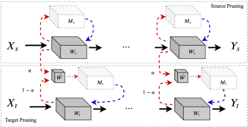
Specifically, we employ a dynamic and cooperative pruning strategy to prune both source and target network simultaneously. We employ a mask matrix consisting of '0's and '1's with the same shape as each layer's parameters to indicate if the parameter at each position should be pruned {0} or kept {1}. The entries in the mask are determined by the absolute values of their corresponding parameters in the full-precision model. In each iteration, parameters are updated by gradient descent: for the parameters pruned by the mask, their gradients are still recorded according to the gradients before penetrating through the mask. The updated parameters lead to a modified mask, which in turn affects the computation in the next iteration. To transfer knowledge, the mask of the target network for each layer is jointly determined by its own parameters and the ones from the source network via a weighted scalar parameter α, named as "transfer factor". Transfer factor α determines how much knowledge is leveraged from the source domain to the target domain. We dynamically set α in the training process to reflect dynamic knowledge transfer. Specifically, α is set larger at the beginning of training because target domain is assumed to rely heavily on source supervision to achieve a good initial state. As training proceeds, we gradually decrease α to allow the target network to learn from itself. We show in the experiment that the dynamic transfer factor could achieve a smooth knowledge transfer for better prediction performance.
Compared with most existing methods, Co-Prune is capable of conducting model pruning in the domain with only limited training data and without a well-trained initial state. Our contributions are listed in the following: 1) Our method can deal with neural network pruning under the scenario of limited training data. 2) We pioneer the idea of knowledge transfer from a resource-rich domain to conduct neural network pruning in target domains. 3) Extensive experiments are conducted to verify the effectiveness of our proposed method compared with several state-of-the-art approaches in the setting of limited training data. Codes are available at https://github.com/csyhhu/Co-Prune.
2 RelatedWork
Element-Wise Pruning. Neural networks pruning has been studied since last century. LeCun et al.[1990] proposed to study training loss difference after pruning one parameter as a criterion to measure its importance. This difference is approximated as the multiplication of some power of the weight's magnitude and its Hessian. Hassibi and Stork[1993] modified this measurement by incorporating the updates of the other weights to compensate for pruning. Entering the era of deep learning, Han et al.[2015] proposed to measure the importance of a parameter by its absolute value in a well-trained model. Dong et al.[2017] adapted [Hassibi and Stork, 1993]'s criterion in deep neural networks in a layer-wise setting by simplfying calculation of the Hessian and proved a theoretical bound for pruning error propagation. The aforementioned methods calculate the importance for each parameter based on a pre-trained model, and conduct pruning by deleting less important parameters while keeping the others. On the contrary, Guo et al.[2016] performed pruning in a training style: during the training of neural networks, it consistently pruning parameters according to its absolute value.
Domain Adaptation. Domain adaptation [Pan and Yang, 2010] aims at training a model for a target domain where labeled data is unavailable or scarce, with the assistance of a source domain with abundant data. Tzeng et al.[2014] extended the idea of transfer component analysis (TCA) [Pan et al., 2011] in the context of deep neural networks. Following the similar idea of reducing discrepancy of source and target features, Ganin and Lempitsky[2014] and Tzeng et al.[2017] introduced a discriminator to distinguish both domains, while training both models to cheat the discriminator. However, most domain adaptation methods focused on performance improvement in full-precision models for target domain, without considering knowledge transfer to assist model compression.
Knowledge Distillation. Distillation is commonly used in knowledge transfer, where information from a large model (denoted as "teacher") is delivered to a small and compact model ("student") [Bucilua et al., 2006]. Hinton et al.[2015] formulated this process by minimizing the difference between outputs of these two networks given the same inputs. Romero et al.[2014] proposed to improve knowledge transfer by matching the features in middle layers. Gupta et al.[2016] studied knowledge transfer between two models: RGB images to paired depth image, by teaching the network to reproduce the mid-level semantic representations. However, most distillation methods aim at transferring knowledge to a compact or shallow models, which may lack ability to store all the information. Pruning focuses on finding the redundant connections in large models and provide regularization, which is used in Co-Prune to provide better knowledge transfer.
3 Cooperative Pruning
Given a pre-trained neural network model in terms of Ws, a training dataset Ds with ns data from the source domain, and a limited training dataset Dt with nt data from the target domain, we aim to produce a pruned model W′t = WtMt for the target domain, where Wt denotes the target-domain full-precision network, which is unknown at the beginning, W′t parameterizes the target-domain network after pruning, and Mt is the mask matrix. Normally, the target dataset is less than 1/10 of the source dataset which is insufficient to train a good deep neural network model. For each layer of a model, a mask matrix (M) of the same shape as model parameters is introduced to indicate whether a parameter is pruned or not (denoted by 0 or 1). We preserve two networks and their mask matrices for the source domain (Ws, Ms) and the target domain (Wt, Mt), respectively. Wt is initialized from the fine-tuned model in the target domain trained fromWs. The marks Ms and Mt are initialized with all 1's. During training, bothWs andWt are updated through gradient descent, while Ms and Mt are directly computed accordingly. We update Ws during training to dynamically affect Mt. A Compression Ratio (CR) is set for each layer to control the percentage of remaining parameters after pruning.
Fig.1 illustrates a sketch architecture for Co-Prune: Pruning is conducted by imposing layer-wise pruning mask for model's parametersWs (Wt). During training, the maskMs (Mt) is updated in each iteration according to current value of parameters, which is explained in detail in Sec.3.1. Pruning mask Ms for the source domain is independently generated from its own parameters, as in (3). For the target domain, the pruning mask Mt is obtained from the parameters of both source and target networks via (5), where knowledge from the source domain is selectively transferred to the target domain.
3.1 Mask Generation
It is rather difficult to train a target model from scratch using only limited target data. On the other hand, directly applying and fine-tuning the pre-trained model from a source domain for target predictions is not feasible due to large domain shift. Therefore, we propose to leverage information from the source model to assist target predictions through cooperative mask generation. We regard the mask as the bridge connecting source/target domain and transferring knowledge between them. Specially, given parameters W, masking function (M) and its leading mask M is defined as:
where Imp(·) is a function measuring parameters' importance. For example, [LeCun et al., 1990] defined it as: Imp(w) = ∂ 2L ∂w2 ×w2 , involving hessian of each parameter and its square. In Co-Prune, to efficiently calculate parameters' importance, it is defined as: Imp(Wi,j) = |Wi,j|. σImp(CR) represents a mapping from parameters (with n elements) to pruning threshold given Imp(·) and CR set for this layer:
Increasing(W, i) takes out the i-th element of an increasing ranking of elements from Imp(W).
The mask for each layer of source parameters Ws is generated using (1) independently:
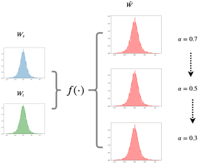
The mask matrix embeds information about parameters' importance in each domain. We assign a scalar variable α, named as "transfer factor" to control the knowledge flow by a fusion function f(Ws,Wt, α) for generating the mask in the target domain. In Co-Prune, transfer factor produces a weighted sum of both source and target model parameters as the following:
Then ˜W is utilized to compute the mask matrix for target model using (1) as
The pruned positions inMt are set as 0, while the rest are set as 1. During this process, knowledge from the source model is transferred to the target, regulated through α. The mask is imposed into each layer of the network for inference and calculation of loss, which is denoted by:
with d ∈ {s, t}, where ⊙ represents element-wise multiplication betweenWd andMd.
3.2 Adaptive Domain Adaptation via Transfer Factor α
Cooperative pruning can be regarded as source model (teacher) transferring knowledge to target model (student). Because of limited data in the target domain, learning at the beginning requires more guidance from the source domain by exploring the commonalities across different domains. As training proceeds, it is assumed that the target model is capable of learning more domain-dependent information from itself. This dynamic mechanism is implemented by adjusting α: assigning a large α at the beginning, and reducing it gradually along with the training process. Specially, in CoPrune a non-increasing discrete function for αk w.r.t iteration of training optimum k is defined:
α0 is the initial factor, αmin is the minimal value that αk can reach. When training comes at optimum using current αk, it will be updated by (7) to obtain αk+1. β represents sensitivity of {αk}. In Co-Prune, α0 = 0.7, αmin = 0.3, β = 3 for tradeoff between computational time and accuracy. Further studies on how to choose α0, αmin and β are experimented in Sec4.2.
As shown in Fig. 2 for an example of adaptive α: parameters from source and target are weighted summed by a gradually changing α, leading to combined parameters with the importance of each domain weighed by α.
3.3 Training-based Pruning
Traditional pruning is conducted in a "Prune-Retrain" fashion: Firstly, prune less important paramters based on the pretrained model by corresponding Imp(·), then retrain the remaining parameters while fixing the pruned ones. Such onetime pruning strategy fails to retrieve pruned parameters that appear to be essential in a latter training stage. This could be the case in cross-domain pruning: some weights need to be retrieved in the source model to be adapted to the target model. Compared to direct pruning, imposing a mask matrix over parameters to perform pruning is a better way to keep original parameters.
However, when conducting backward update, the gradients of those parameters with 0 mask values are 0, making it similar to one-time pruning. To overcome this limitation and enable model adaptation during cross-domain training, we borrow the idea of "straight-through estimator" (STE) from neural network quantization: For non-differentiable quantization function Q imposed on value r to obtain q = Q(r), the gradient of loss w.r.t q is attained as ∂C ∂q = gq. The straight-through estimator of ∂C ∂r = gr is simply: gr = gq1|r|≤1.
Specially, during inference, consider that pruning function is conducted on W, leading to ˆW = M ⊙ W = M(W) ⊙W. where we omit subscripts {s, t} for the ease of illustration. During inference, loss of neural network is:
For backward computation, assume that gradient of Lw.r.t ˆW is attained as g ˆW = ∂L ∂ ˆW . In Co-Prune, estimator of gW = ∂L ∂W is obtained by
During training-based pruning, each layer consists of a Compression Ratio (CR) that is set heuristically, representing the proportion of the remaining parameters. After parameter updates using (9) in each iteration, Parameters below the threshold attained by (2) are pruned by setting the corresponding positions in the mask matrix as 0 for this iteration, as indicated in (1). In the subsequent training iterations, pruned parameters can be recovered according to their persistent update as (9). This training-based pruning enables 1) parameter recovery to optimize final performance and 2) model adaptation when applying the model on target data.
3.4 Algorithm and Implementation Details
Alg.1 illustrates the whole process of Co-Prune: Source and target models are trained using their corresponding data and current masks. Masks are updated accordingly with the updates of model parameters by (3) and (5). In practice, Adam [Kingma and Ba, 2014] with initial learning rate 10-3 is used for Co-Prune and all retraining processes. Learning rate will be divided by 10 when training loss increases for 3 consecutive epochs. Training to optimum is considered as learning rate becomes smaller than 10-6 .
4 Experiment
To simulate practical scenario, two datasets with abundant source data and limited target data are utilized.
Algorithm 1 Co-Prune
Require: Source training data Ds = {Xs, Ys}ns , target training data Dt = {Xt, Yt}nt , source pre-trained model Ws
Ensure: Final target modelWt and maskMt.
Initialize source model using Ws, target model as target fine-tuned model based on Ws, source-specific mask Ms, target-specific mask Mt with all 1s. α = α0
while α ≥ αmin do while Not Optimum do Train Ws using Ds and Ms, Wt using Dt and Mt by (8) and (9). Update mask Ms by (3). Update mask Mt by (5). end while α is tuned by (7). end whileCIFAR9-STL9 is a modified version of combined CIFAR10 and STL10 dataset. CIFAR10 is a classical 10-class dataset with 50000 32 × 32-pixel training data. Inspired by this dataset, STL10 is designed with 10 similar classes that consists of very limited labeled samples: 5000 96 × 96-pixel training data. We exclude one class from CIFAR10/STL10 that is not shared in both datasets and name the resulting data as CIFAR9/STL9. After exclusion, we treat CIFAR9 as the source domain and STL9 as the target domain.
ImageCLEF is a 4-domain image dataset. It extracts 600 images of 12 classes from ImageNet [Deng et al., 2009], Caltech-256 [Griffin et al., 2007], PASCAL [Everingham et al., 2010] and Bing, respectively. We regard ImageNet dataset as the source domain. Specifically, an ImageNet pretrained model is downloaded online. Then the last layer is replaced with a 12-output fully-connected layer in order to be used for 12-class classification problem. We use the 600image ImageNet data to finetune the whole model, which is utilized as the source pre-trained model. The rest three datasets in ImageCLEF are regarded as target domains.
To verify Co-Prune's generalization ability, we experiment with CIFAR-Net [Jia et al., 2014] in CIFAR9-STL9, ResNet18 [He et al., 2016] in ImageCLEF. For CIFAR-Net, CR of each layer is set manually. For ResNet18, a unified CR is set for every layer.
4.1 Comparison Experiment
We conduct comparison experiments using the following baseline pruning methods: 1) LWC [Han et al., 2015], 2) OBD [LeCun et al., 1990], 3) DNS [Guo et al., 2016], 4) LOBS [Dong et al., 2017]. LWC measured parameters' importance using their absolute value. OBD used hessian and their squared value to indicate the parameters importance. L-OBS formulated pruning for each layer as an optimization problem, which is solved to attain parameters' sensitivity. Given a pre-trained model, these three methods performed one-time pruning according to their measurement of weights' importance. A retraining process is then conducted while fixing the pruned weights. DNS performed pruning in a dynamic way: after parameters updates, their importance will be recalculated by their corresponding absolute values, then parameters are pruned under certain probability related to the importance. Since these methods are not designed specifically for cross-domain pruning, to make fair comparison, all methods firstly retrain the target model based on provided pre-trained model in the source domain as an initial state. Then target data is utilized for the pruning process.
Besides, we use a classical domain adaptation algorithms with modification for pruning as baselines from perspective of domain adaptation: DDC [Tzeng et al., 2014]. DDC trained source and target network with additional minimization of Maximum Mean Discrepancy (MMD) distance of intermediate features. To revise DDC for pruning with supervised domain adaptation, we use DNS networks as target network, with additional target label loss to assist training. We name it as DDC-DNS.
Since data is quite limited in ImageCLEF, we divide each domain into 80% for training and 20% for testing (with class balance). Every experiment are conducted 10 times with random data partition. For each partition, performance improvement with variance of each method is recorded.
| CR (%) | Method | FP Acc (%) | Prune Acc (%) |
|---|---|---|---|
| 10.4 | LWC OBD | 68.03 | 66.26 |
| 65.78 | |||
| DNS | 66.25 | ||
| L-OBS | 66.01 | ||
| DDC-DNS | 66.49 | ||
| Co-Prune | 66.99 | ||
| LWC | 57.47 | ||
| OBD | 50.82 | ||
| DNS | 58.89 | ||
| 1.3 | L-OBS | 56.00 | |
| DDC-DNS | 56.79 | ||
| Co-Prune | 60.5 | ||
| One-Time Co-Prune | 55.36 | ||
| Distillation | 53.16 | ||
| LWC | 49.53 | ||
| OBD | 48.34 | ||
| 0.9 | DNS | 53.32 | |
| L-OBS | 53.04 | ||
| DDC-DNS | 47.86 | ||
| Co-Prune | 56.21 |
We compare Co-Prune with LWC, OBD, DNS, L-OBS, DDC-DNS in CIFAR9-STL9 using CIFAR-Net under different CRs. Table.1 illustrates performance of the pruned model under different methods: Co-Prune outperforms all baseline methods in all selected CR. Especially, as CR decreases, CoPrune shows more obvious advantage over other methods.
To validate the effect of training-based pruning used in CoPrune, which differentiates from one-time pruning in that: pruning strategy is changing during training. We conduct an experiment of Co-Prune using one-time pruning (named as "One-Time Co-Prune") in Table.1, specially, mask is updated only at the beginning of training. The performance drops significantly from 60.5% to 55.36%. This demonstrates that training-based pruning contributes to Co-Prune.
Comparison experiments with non-pruning compression is conducted using distillation. We construct a slim CIFARNet which contains 10.4% parameters of the original one. This slim network is trained by ground-truth and distilled from original target-retrained CIFARNet (who is retrained using target data based on source pre-trained network). As Table.1 shows it reaches 53.16%, worse than Co-Prune.
| Direction | Method | FP Acc (%) | Improve Acc (%) |
|---|---|---|---|
| I→P | LWC OBD | 60.917±3.809 | -16.167±3.617 -28.333±7.188 |
| DNS | -11.417±3.556 | ||
| L-OBS | -8.317±3.435 | ||
| DDC-DNS | -12.917±4.075 | ||
| Co-Prune | -6.583±3.525 | ||
| I→C | LWC | 87.417±2.898 | -6.833±3.851 |
| OBD | -30.500±14.664 | ||
| DNS | -5.583±2.912 | ||
| L-OBS | -5.018±3.214 | ||
| DDC-DNS | -6.167±3.009 | ||
| Co-Prune | -3.083±2.936 | ||
| I→B | LWC | 49.667±3.232 | -11.667±2.609 |
| OBD | -18.250±2.661 | ||
| DNS | -7.667±2.577 | ||
| L-OBS | -8.973±4.735 | ||
| DDC-DNS | -6.500±5.711 | ||
| Co-Prune |
-5.648±3.659
Table 2: Overall results of ImageNet→PASCAL, ImageNet→Caltech256, ImageNet→Bing using ImageNet pre-trained ResNet18. CR is 4% for each layer
Similarly, we conduct 3 cross-domain pruning from ImageNet to PASCAL, Caltech256, Bing, respectively. In Table.2, we compare the performances of different methods in various target domains, using ResNet18 with 4% CR in each layer. For all the cross-domain directions, Co-Prune shows the best average performance over other methods.
4.2 Effect of Transfer Factor α
To examine α's properties in Co-Prune, CIFAR9-STL9 in CIFAR-Net under CR at 1.3 is used as an example.
Variation of Co-Prune. When α=0, Co-Prune reduces to DNS as it only replies on target data to generate mask and conduct training. For α=1, Co-Prune depends on source model to generate mask for target pruning. Total dependence on source or target does harm in finding optimal pruning strategy. As Table.3 shows, Co-Prune with adaptive α outperforms other variations, showing that proper knowledge transfer from source assists in improving pruning on target model.
| α | FP Acc | Prune Acc |
|---|---|---|
| 0 (DNS) | 58.89 | |
| 0.7→0.5→0.3 | 68.03 | 60.5 |
| 1 | 57 |
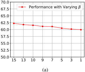
Effect of Sensitivity β. (7) determines the sensitivity of transfer factor. We experiments with various β by fixing α0 = 0.7, αmin = 0.3 and record its best performance in Fig.3(a): Performance of Co-Prune under various β shows changes with mean and variance as 60.91±0.8%, whose Performance with Varying α0
0.9 0.7 0.66 0.63 0.6 0.5 0.3
(b)
Performance with Varying αmin
0.7 0.5 0.4 0.36 0.33 0.3 0.1
(c)
Figure 3: (a) Performance of Co-Prune under various β with fixed α0 = 0.7, αmin = 0.3; (b) Performance of Co-Prune under various α0 with fixed β = 3, αmin = 0.3; (c) Performance of Co-Prune under various αmin with fixed α0 = 0.7, β = 3. Y axis represents the best performance under corresponding setting, X axis represents β, α0, αmin, respectively
average exceeds all baseline methods by a large margin. This result shows that Co-Prune is consistent and stable with different sensitivity when tuning α.
Effect of Initial α0. α0 is set as initial value for transferring knowledge. We examine the effect of this initial state to final performance of Co-Prune. β = 3 and αmin = 0.3 are fixed and the best performance is reported in Fig.3(b). Performance drops when α0 is too large (starting from learning too much from source and intense tuning of α) or too small (starting from learning too few from source). The performance is rather stable when α0 ranges within [0.6, 0.7] and shows better performance.
Effect of Minimum αmin. Co-Prune terminates after training reaches optimum using αmin Effect of this final state to performance of Co-Prune is experimented with β = 3 and α0 = 0.7 fixed. The best performance with various αmin is reported in Fig.3(c). αmin = 0.7 gets the worst performance, which is even lower than DNS. If αmin is getting too large, it means there is almost no changes in α. When αmin is set within [0.3, 0.4], Co-Prune shows the best performance.
4.3 Performance Under Various CRs
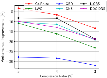
We further study how different methods perform in different CRs. I→P from ImageCLEF using ResNet18 is utilized as an example to verify the performances of different methods from CR: 5% → 4% → 3%. Fig.3(c) illustrates the variation of performance improvement under pruned methods. Among all the methods, Co-Prune performs the best in all CRs.
4.4 Complexity Analysis
We set number of parameters as n, training iteration as T. training-based pruning methods, such as Co-Prune, DNS, their time complexity can be represented as O(t(n+nlogn)). For one-time pruning methods (pruning strategy is determined at the begining), LWC: O(tn+nlogn), OBD: O(tn+ nlogn + n2 ), L-OBS: O(tn + nlogn + D2 ), where D is the size of dataset used in hessian approximation.
5 Conclusion
In this paper, we propose a novel cross-domain pruning algorithm (Co-Prune) for deep neural network. Traditionally, pruning algorithms reply on a well-trained network and a huge amount of training data, which is not realistic in many domains. Co-Prune solves this problem by training-based pruning, with the construction of target's pruning mask that incorporates knowledge from the source domain. An adaptive transfer factor that controls the knowledge flow from the source domain for target pruning is introduced to further boost the performance. Extensive experiments are conducted on two benchmark datasets to demonstrate Co-Prune's performance over baseline methods.
Acknowledgements
This work is supported by NTU Singapore Nanyang Assistant Professorship (NAP) grant M4081532.020.
@inproceedings{ijcai2019p291,
  title     = {Cooperative Pruning in Cross-Domain Deep Neural Network Compression},
  author    = {Chen, Shangyu and Wang, Wenya and Pan, Sinno Jialin},
  booktitle = {Proceedings of the Twenty-Eighth International Joint Conference on
               Artificial Intelligence, {IJCAI-19}},
  publisher = {International Joint Conferences on Artificial Intelligence Organization},
  editor    = {Sarit Kraus},
  pages     = {2102--2108},
  year      = {2019},
  month     = {8},
  note      = {Main track},
  doi       = {10.24963/ijcai.2019/291},
  url       = {https://doi.org/10.24963/ijcai.2019/291},
}
TY - CPAPER TI - Cooperative Pruning in Cross-Domain Deep Neural Network Compression AU - Chen, Shangyu AU - Wang, Wenya AU - Pan, Sinno Jialin T2 - Proceedings of the Twenty-Eighth International Joint Conference on Artificial Intelligence, IJCAI-19 PB - International Joint Conferences on Artificial Intelligence Organization PY - 2019 SP - 2102 EP - 2108 DO - 10.24963/ijcai.2019/291 UR - https://doi.org/10.24963/ijcai.2019/291 ER -Copied
Machine-readable versions of this paper, for tools and AI agents:





