
STCA: Spatio-Temporal Credit Assignment with Delayed Feedback in Deep Spiking Neural Networks
Proceedings of the Twenty-Eighth International Joint Conference on Artificial Intelligence. Main track. Pages 1366-1372.
https://doi.org/10.24963/ijcai.2019/189
Keywords
- Humans and AI: Cognitive Modeling
Abstract
The temporal credit assignment problem, which aims to discover the predictive features hidden in distracting background streams with delayed feedback, remains a core challenge in biological and machine learning. To address this issue, we propose a novel spatio-temporal credit assignment algorithm called STCA for training deep spiking neural networks (DSNNs). We present a new spatiotemporal error backpropagation policy by defining a temporal based loss function, which is able to credit the network losses to spatial and temporal domains simultaneously. Experimental results on MNIST dataset and a music dataset (MedleyDB) demonstrate that STCA can achieve comparable performance with other state-of-the-art algorithms with simpler architectures. Furthermore, STCA successfully discovers predictive sensory features and shows the highest performance in the unsegmented sensory event detection tasks.
- [Bittner et al., 2014] Rachel Bittner, Justin Salamon, Mike Tierney, Matthias Mauch, Chris Cannam, and Juan Bello. Medleydb: A multitrack dataset for annotation-intensive mir research. In ISMIR, 2014.
- [Diehl and Cook, 2015] Peter U Diehl and Matthew Cook. Unsupervised learning of digit recognition using spike- timing-dependent plasticity. Frontiers in computational neuroscience, 9:99, 2015.
- [Diehl et al., 2015] Peter U Diehl, Daniel Neil, Jonathan Bi- nas, Matthew Cook, Shih-Chii Liu, and Michael Pfeif- fer. Fast-classifying, high-accuracy spiking deep networks through weight and threshold balancing. In IJCNN, pages 1-8. IEEE, 2015.
- [Esser et al., 2015] Steve K Esser, Rathinakumar Ap- puswamy, Paul Merolla, John V Arthur, and Dharmen- dra S Modha. Backpropagation for energy-efficient neuromorphic computing. In NIPS, pages 1117-1125, 2015.
- [Gerstner et al., 2014] Wulfram Gerstner, Werner M Kistler, Richard Naud, and Liam Paninski. Neuronal dynamics: From single neurons to networks and models of cognition. Cambridge University Press, 2014.
- [Grüning and Bohte, 2014] André Grüning and Sander M Bohte. Spiking neural networks: Principles and chal- lenges. In ESANN, 2014.
- [Gütig, 2016] Robert Gütig. Spiking neurons can discover predictive features by aggregate-label learning. Science, 351(6277):aab4113, 2016.
- [Jin et al., 2018] Yingyezhe Jin, Wenrui Zhang, and Peng Li. Hybrid macro/micro level backpropagation for training deep spiking neural networks. In NIPS, pages 7005-7015, 2018.
- [LeCun et al., 1998] Yann LeCun, Léon Bottou, Yoshua Bengio, Patrick Haffner, et al. Gradient-based learning ap- plied to document recognition. Proceedings of the IEEE, 86(11):2278-2324, 1998.
- [Lee et al., 2016] Jun H Lee, Tobi Delbruck, and Michael Pfeiffer. Training deep spiking neural networks using backpropagation. Frontiers in neuroscience, 10:508, 2016.
- [Nakamura et al., 2000] Satoshi Nakamura, Kazuo Hiyane, Futoshi Asano, Takanobu Nishiura, and Takeshi Yamada. Acoustical sound database in real environments for sound scene understanding and hands-free speech recognition. In LREC, 2000.
- [Neftci et al., 2017] Emre O Neftci, Charles Augustine, Somnath Paul, and Georgios Detorakis. Event-driven random back-propagation: Enabling neuromorphic deep learning machines. Frontiers in neuroscience, 11:324, 2017.
- [Neil et al., 2016] Daniel Neil, Michael Pfeiffer, and Shih- Chii Liu. Learning to be efficient:algorithms for training low-latency, low-compute deep spiking neural networks. 2016.
- [Pons et al., 2017] Jordi Pons, Olga Slizovskaia, Rong Gong, Emilia Gómez, and Xavier Serra. Timbre analysis of music audio signals with convolutional neural networks. In EUSIPCO, pages 2744-2748. IEEE, 2017.
- [Qi et al., 2018] Yu Qi, Jiangrong Shen, Yueming Wang, Huajin Tang, Hang Yu, Zhaohui Wu, and Gang Pan. Jointly learning network connections and link weights in spiking neural networks. In IJCAI, pages 1597-1603, 2018. IJCAI
- [Samadi et al., 2017] Arash Samadi, Timothy P. Lillicrap, and Douglas B. Tweed. Deep learning with dynamic spik- ing neurons and fixed feedback weights. Neural Compu- tation, 29(3):578-602, 2017.
- [Smith and Lewicki, 2005] Evan Smith and Michael S Lewicki. Efficient coding of time-relative structure using spikes. Neural Computation, 17(1):19-45, 2005.
- [Tavanaei and Maida, 2019] Amirhossein Tavanaei and An- thony Maida. Bp-stdp: Approximating backpropagation using spike timing dependent plasticity. Neurocomputing, 330:39-47, 2019.
- [Werbos, 1990] Paul J Werbos. Backpropagation through time: what it does and how to do it. Proceedings of the IEEE, 78(10):1550-1560, 1990.
- [Wu et al., 2018] Yujie Wu, Lei Deng, Guoqi Li, Jun Zhu, and Luping Shi. Spatio-temporal backpropagation for training high-performance spiking neural networks. Fron- tiers in neuroscience, 12, 2018.
- [Xu et al., 2018] Qi Xu, Yu Qi, Hang Yu, Jiangrong Shen, Huajin Tang, and Gang Pan. Csnn: An augmented spik- ing based framework with perceptron-inception. In IJCAI, pages 1646-1652, 2018. IJCAI
- [Yu et al., 2018] Qiang Yu, Haizhou Li, and Kay C Tan. Spike timing or rate? neurons learn to make decisions for both through threshold-driven plasticity. IEEE Transac- tions on Cybernetics, 2018.
- [Zhang et al., 2018] Tielin Zhang, Yi Zeng, Dongcheng Zhao, and Mengting Shi. A plasticity-centric approach to train the non-differential spiking neural networks. In AAAI, 2018.
References were extracted automatically from the PDF and may contain errors.
Full text extracted automatically from the PDF; figures, tables and equations may differ. The PDF is the version of record.
1 Introduction
In dynamic environments, the useful sensory features are always embedded in distracting streams of unrelated sensory activity. Even worse, the feedback events that the features predict may happen after long and variable delays. To discover these features, a learning model needs to amplify the correlations between features and the delayed feedback. This temporal credit assignment (TCA) problem is challenging in both biological and machine learning.
One potential solution for this problem is utilizing SNNs to learn the temporal information of sensory streams. SNNs are proposed to capture the temporal dynamics of neural behaviors. They use discrete and binary spike trains in which the precise spike times are significantly informative [Gerstner et al., 2014] to convey information, so they are more biologically realistic than artificial neural networks (ANNs) and thus gain increasing interest in recent years.
Recently, several spiking models [G¨utig, 2016; Yu et al., 2018] are proposed to solve this problem based on the intuition: a spiking neuron which is a neural detector of a sensory clue should fire spikes whenever the predictive features occur but remain silent otherwise [G¨utig, 2016]. A spiking neuron was trained to match their spike activities with the clue's number of occurrences. As a result, the neuron can identify an unknown feature without knowing the specific timing when the desired feature occurs. These approaches use a threshold-driven learning strategy to reduce the discrepancy between the output neuron's actual threshold and the closest hypothetical threshold at which the neuron would fire a desired number of spikes. However, finding the hypothetical threshold is computationally complex and time-consuming. Furthermore, they are limited to train single-layer SNNs and thus cannot be applied to complex tasks.
∗Corresponding author: huajin.tang@gmail.com
While there exist many models of single-layer SNNs [Xu et al., 2018; Qi et al., 2018], the complex temporal dependencies of spiking neurons and non-differentiable property of binary spike function [Wu et al., 2018] both make training DSNNs difficult. For instance, the ANN-to-SNN approaches [Neil et al., 2016; Diehl et al., 2015] usually leverage conventional learning methods to train an ANN and convert it into an SNN. They rely on carefully designed techniques to techniques to overcome the loss of accuracy caused by conversion, such as using probabilistic weights [Esser et al., 2015], adding constraints on neuron firing rate [Diehl et al., 2015] and so on. Some works [Lee et al., 2016; Samadi et al., 2017] only propagate the error back to preceding layers without considering the temporal dependencies of spiking neurons. They require other mechanisms to keep the performances stable, such as lateral inhibition, error normalization, parameter regularization, etc. [Wu et al., 2018] propose a method to directly derive the spatio-temporal gradients for DSNNs. It captures the temporal effects of spikes by performing BPTT [Werbos, 1990] and utilizes surrogate derivatives to handle spiking discontinuities. [Jin et al., 2018] computes the gradients across both rate and temporal level by establishing the relationship between firing rate and synaptic potential. The loss functions of the above algorithms are all rate-based. While they can offer good performance, they lose the temporal information embedded in output spike trains, which is crucial for the TCA problem.
In this paper, we firstly propose a novel loss function based on the definition of "spike cluster" to assign the network loss to the voltage at a specific time point and then introduce an iterative policy to backpropagate the error signal to spatial and time domains simultaneously. This algorithm shows excellent generalization performance on both classification and TCA problems. As demonstrated in experimental results, its performance on MNIST dataset outperforms most of the existing DSNNs. It also gets a comparable result with a specialized convolutional neural network (CNN) on a music dataset (MedleyDB) by using a much simpler architecture. In the unsegmented sensory event detection tasks, it successfully discovers the embedded events and outperforms the state-of-theart method.
2 NeuronModel and Learning Algorithm
In this section, we first present a spiking neuron model and its iterative computation mechanism used in this work. Then, we propose a novel loss function which yields a more flexible temporal credit assignment. Finally, we present an iterative procedure to backpropagate the error signal to spatial and temporal domains simultaneously.
2.1 Spiking NeuronModel
Here, we adopt the current-based leaky integrate-and-fire (CLIF) neuron model [G¨utig, 2016] as the basic computational units in DSNNs. The C-LIF model is biologically realistic and mathematically tractable. Its voltage trace V (t) can be expressed as:
where (M(t) - S(t)) describes that the neuron integrates its synaptic current by receiving input spikes from N presynaptic neurons, and E(t) indicates that each output spike will refrain the voltage for a while. Here, tkj is the time of the k-th input spike from the j-th afferent neurons; ti denotes the time of the i-th output spike; wij is the synaptic weight; τm, τs are the time constants; V0 is a normalization factor; ϑ denotes the threshold of the neuron.
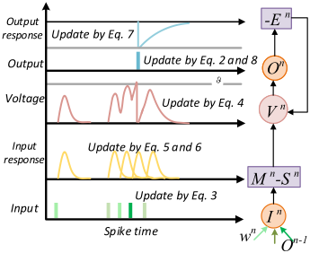
Most works [G¨utig, 2016; Yu et al., 2018] based on C-LIF model merely use Eq. (1) to derive their training algorithms. This makes them difficult to develope error backpropagation in DSNNs. Because Eq. (1) neither completely captures the temporal dependency in the spiking neuron nor reveals the explicit relationship between the input spike signals ejected from the preceding layer and the output spike train of the current neuron. To solve this problem and ensure computational tractability, we discretize the temporal system with a sampling time dt and thus replace t and V (t) with k · dt and V [k] = V (k · dt), where k ∈ Z. Then, an iterative mechanism is presented to capture the spatio-temporal dynamics of C-LIF neuron (Figure 1) according to its event-driven property [Yu et al., 2018; Wu et al., 2018]:
These fomulas are explanied as follow:
- The upper index n, subscript i, and k indicate that the variable is a state of the i-th neuron at the n-th layer and the k-th time point. L(n) indicates the number of neurons in the n-th layer.
- On i [k] ∈ {0, 1} is the output signal of the neuron. It is governed by the spike function g(.) (Eq. (8)). On i [k] = 1 indicates a spike activity, On i [k] = 0 denotes nothing occurs.
- I n i [k] is the input weighted summation of the spike signals On-1 j [k] which are generated from the previous layer.
- V n i [k] is the superposition of the input response (M n i [k] - Sn i [k]) and the output response -En i [k]. It represents the voltage of neuron.
- M n i [k], Sn i [k],En i [k] are all expressed by their states at the (k - 1)-th time step. Further, M n i [k], Sn i [k] are also governed by the input signal at the k-th time step, while En i [k] is governed by the output signal at the (k - 1)-th time step.
- βm(s) = exp(- dt τm(s) ) < 1 are the decay factors. If no spike occurs, the input response and output response will decay to 0 by multiplying decay factors recursively.
2.2 Temporal-based Loss Function
To solve the TCA problem, we draw inspirations from the recent work [G¨utig, 2016] and its intuition: when a neuron is trained to match its number of output spikes to the magnitude of the occurrence number of sensory events, it will identify the sensory clues whose occurrences predict the delayed feedback.
The original loss function in [G¨utig, 2016] will train the neuron to fire a fixed number of spikes after detecting a desired event. Indeed, this objective seems inflexible and unreasonable. Because spiking neurons tend to fire a different number of spikes if they receive distinct input activities. However, there might exist distinct features among the activities from the same class. Under this case, forcing the neurons to issue a fixed number of spikes will lead to an unstable performance of the network. To address this problem, we introduce a novel definition as follow:
- Spike cluster: If the intervals between any adjacent spikes in a spike train C are less than a predefined constant Tin, and the intervals between spikes in C and other outside spikes are greater than Tin, we define C as a spike cluster.
Utilizing this definition, we can set a more flexible objective for the output spiking neuron: when the predictive features are recognized, the neuron should issue one spike cluster instead of a fixed number of spikes. Hence, the goal of our loss function is to make the actual number of spike clusters No equals to the number of desired features Nd.
However, directly defining |Nd -No| as our loss function will evenly assign error to all states of the neuron over the entire time window. This is not conducive and convenient to find the predictive features which usually occur within short epochs. Therefore, we introduce a temporal based loss function to assign the error to the voltage of a specific time point which may well be related to the desired features. The specific time point can be found by two strategies as follow:
- When No < Nd, the neuron does not identify all desired features. In this case, the time point k+ is most likely associated with the desired features which is not identified, as V N [k+] is the highest maximum of subthreshold voltage and outside the occurrence epoch of any spike cluster (Figure 2). Hence, the objective is to potentiate V N [k+] towards the threshold ϑ with the aim of firing more spike clusters.
- When No > Nd, it indicates that the neuron has identified the undesired features. In this case, the undesired features may well be associated with the spike cluster which has the fewest number of spikes. Thus, we credit the loss to V N [k-] in order to depress V N [k-] falling below ϑ with the purpose of removing the wrong spike cluster, as k- is the last spike time of the spike cluster whose spike number is the fewest (Figure 2).
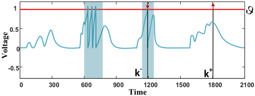
Both of the strategies are effective because they can find the time point k∗ quickly by traversing the voltage trace once (k∗ is the gerneral term for the k+ and k-). The temporal based loss function can be written as follow:
where N is the index of the output layer. It is also easy to generalize this function into classification tasks. Expecting that neuron will fire one or more spike cluster when the sample label ys = 1 but keep silent otherwise, we can define L as follow:
2.3 Spatio-Temporal Credit Assignment Policy
To backpropagte the error signal at V N [k∗ ] to preceding layers (<= N) and previous time points (<= k∗ ) accurately, we unfold the states of C-LIF neurons on both spatial and temporal domains as illustrated in Figure 3. By this way, we can explicitly observe how each variable contributes to other variables (indicated by arrows) along the spatial direction and temporal direction and can compute gradients iteratively by performing BPTT [Werbos, 1990].
We first denote ∂L ∂I n [k] and ∂L ∂V n [k] as δn [k] and ϵn [k] respectively. δn [k] can be computed as follow:
When k < k∗ , M n [k] contributes to M n [k + 1] and V n [k] directly, so we can get its derivative by:
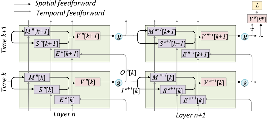
In the same way, we can get:
To handle the non-differentiable property of g(.) which causes the gradient vanishing or exploding problem, we adopt the rectangular function h(.) mentioned in [Wu et al., 2018] to be surrogate of the derivative of g(.):
where α is a constant to determine the width of h(.). The approximation of ϵn [k] will be different in two cases:
- When n = N, V N [k] governs the output response EN [k + 1] by affecting the output activity ON [k], so ϵN [k] can be given by:
- When n < N, the output signal On [k] governed by V n [k] not only contributes to En [k + 1] but also influences the input signal I n+1 [k] at the next layer, it yeilds:
According to Eq. (11-17), the network loss L can be backpropagated from V N [k∗ ] to δn [k] recursively. Note that δn [k] are the gradients of the input signals across all preceding layers (n ∈ [2,N]) and previous time points (k ∈ [1, k∗ ]). Further, the gradients of synaptic weights can be computed as:
The pseudo code is given in Algorithm 1 and our GPU accelerated software implementation is available online 1 .
3 Experimental Results
We demonstrate the advantages of our algorithm by three experiments. Detailed experimental settings (e.g. hyperparameters, error bars, and the convergence curve) are reported in the released online materials 1 .
3.1 MNIST Image Classification
To encode images in MNIST dataset [LeCun et al., 1998], we utilize the rate coding method [Gr¨uning and Bohte, 2014] to convert each image into 784 spike trains whose spiking firing rates equal their corresponding pixel values.
Table 1 lists the state-of-the-art results of the fullyconnected DSNNs with accuracy shown in a descending order. While MNIST is a toy benchmark dataset, and there is no TCA problem in it. Our model still goes beyond the performance of most models by a simpler structure and achieves a comparable result with the optimal model. Furthermore, there are several advantages of STCA over other methods. Firstly, STCA is capable of training DSNNs directly, while the ANN-to-SNN approaches require many converting techniques. Secondly, STCA considers the spatio-temporal effects of spikes during training, while the spiking-BP only Algorithm 1 The training procedure of STCA in one iteration Input: The input spike signals O1 ; the desired number of spike clusters Nd.
1 https://github.com/Squirtle-gpj/STCA-DSNN
Parameter: The number of all layers N; The number of all time points K.
Output: Update the weights w
- 1: //Feedforward: 2: for n = 2 to N do 3: M n [0], Sn [0],En [0],On [0] = 0 // Initialization 4: for k = 1 to K do 5: Compute V n [k],On [k] // Eq. (2 - 8) 6: end for 7: end for 8: //Loss: 9: Get the actual number of spike clusters No. 10: Find the time point k∗ and compute L. // Eq. (9) 11: //Backpropagation: 12: for n = N to 2 do 13: for k = k∗ to 1 do 14: ⋆ Compute ϵn [k] //Eq. (16) or Eq. (17) 15: ⋆ Compute ∂L ∂Mn [k] , ∂L ∂Sn [k] , ∂L ∂En [k] //Eq. (12-14) 16: Compute δn [k] //Eq. (11) 17: end for 18: Compute ∇wn //Eq. (18) 19: end for
- 20: Update all weights based on their gradients.
⋆: The equations to derive ϵn [k∗ ], ∂L ∂Mn[k∗] , ∂L ∂Sn[k∗] , ∂L ∂En[k∗] are slightly different from Eq. (16-17) and Eq. (12-14). They can be derived easily by removing the first terms of the original equations, since the variables at k∗ are not required to receive the error signal from the next time.
considers the spatial effects and thus requires many other optimization techniques. Finally, we utilize the output response
-E to simulate the refractory period of biological neurons. This mechanism can be regarded as a normalization mechanism, since it can prevent spiking neurons from firing too many spikes, and thus the spike representations in the hidden layers are more sparse and effective. In contrast, STBP and HM2-BP do not involve this mechanism.
| Method | # units | Accuracy |
|---|---|---|
| STBP [Wu et al., 2018] | 800 | 98.89 |
| HM2-BP [Jin et al., 2018] | 800 | 98.88 |
| Spiking-BP [Lee et al., 2016] | 800 | 98.71 |
| STCA [Our model] | 800 | 98.60 |
| ANN-to-SNN [Diehl et al., 2015] | 500-300 | 98.60 |
| VPSNN [Zhang et al., 2018] | 4500 | 98.52 |
| ANN-to-SNN [Neil et al., 2016] | 1200-1200 | 98.00 |
| eRBP [Neftci et al., 2017] | 200-200 | 97.98 |
| BP-STDP [Tavanaei and Maida, 2019] | 500-150 | 97.20 |
| LIF-BA [Samadi et al., 2017] | 630-370 | 97.05 |
| STDP [Diehl and Cook, 2015] | 5000 | 95.00 |
3.2 Musical Instrument Recognition
In this experiment, we train a DSNN to identify different instruments in various music pieces which are diverse in melodies and styles. We use the MedleyDB dataset [Bittner et al., 2014] which contains 122 multi-tracks annotated with instrument activations. We extract the monophonic stems corresponding to 10 instruments ('violin', 'guitar', 'flute', 'female', 'drum', 'cymbal', 'cello', 'double bass', 'erhu') and slice them into 1.5s long pieces. For each instrument, we randomly collect 160 pieces as training samples and 80 pieces as test samples.
In Table 2, we use recall, precision, and F1 score to evaluate our model and other three models. Our model gets a comparable result with the specialized CNN whose convolutional kernels' structures are carefully designed for learning timbre representations [Pons et al., 2017]. Additionally, the number of trainable parameters in our model is almost one third of the CNN parameters. Furthermore, our model also outperforms a 3-layer recurrent network. In this network, the first layer receives the spectrogram sequences, and the next two layers are an LSTM layer and a dense layer with softmax activation, respectively. For comparison, we construct this architecture (96-218-10) for this network to make its number of trainable parameters equal to ours. We also consider a DSNN model [Samadi et al., 2017] which doesn't consider the temporal dependencies of spiking neurons during training to verify whether the ability of DSNN to learn temporal features can be improved by assigning network error along the temporal direction. Additionally, our model shares the same network structure (384-700-10) and encoding method with this model, and the encoding method called spikegram [Smith and Lewicki, 2005] which converts the input sound signal into a spike pattern capturing the time-frequency information of sound by the spatio-temporal distribution of spikes. As illustrated, the disappointing performance of this model reveals that error backpropagation on time domain notably promotes SNNs to learn dynamic features.
3.3 Unsegmented Sensory Event Detection
In dynamic environments, it's easy to get a lot of unsegmented sensory streams containing various sensory events. However, the precise occurrence time of individual event is usually unavailable. The temporal alignment with these events requires heavy labor or complex algorithms. To demonstrate that our model can successfully detect the desired events from unsegmented streams, we construct several unsegmented sound event streams by splicing individual sound events extracted from the RWCP dataset [Nakamura et al., 2000]. The RWCP dataset gives a selection of isolated sound event samples in duration around 0.5-3s. Here, 10 classes of sound events are extracted ('bank', 'bells5', 'bowl', 'cherry1', 'coin3', 'cup1', 'horn', 'phone4', 'ring', 'whistle1', each class has 80 samples) and encoded into spikegrams [Smith and Lewicki, 2005]. To construct an unsegmented stream, we will radomly select 5 individual events and spliced together. We extract half of event samples to construct 3000 individual streams as the training set while the rest samples are assigned as the testing set. The occurrence number of the target event in this stream will be used as the desired number of spike clusters. The architecture of our model is 128-30010.
| Model | Encoding method | #params | Recall (%) | Precision (%) | F1 score (%) |
|---|---|---|---|---|---|
| Specialized CNN [Pons et al., 2017] LSTM | Spectrogram | 76.9k 27.6k | 99.21 93.31 | 95.94 96.08 | 97.51 94.62 |
| DSNN [Samadi et al., 2017] Our model | Spikegram | 27.6k 27.6k | 86.56 97.29 | 75.62 97.23 | 80.73 97.25 |
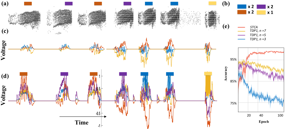
Figure 4 demonstrates the learning effect of STCA. We also compare STCA with TDP1 [Yu et al., 2018] which is the state-of-the art model for solving the TCA problem by plotting their learning curves on the testing set (Figure 4(e)). Our model shows a higher performance than TDP1. The reason is that the objective of TDP1 is to fire a desired number of spikes, which is unreasonable to TCA problem by ignoring the differences between intra-class features and makes the model unstable and even induces a reduction on recognition accuracy. In contrast, the objective of STCA is to fire a desired number of "spike clusters", which is a significant advantage as training on spike cluster is more flexible and less sensitive to input data than training on indivuidual spikes. Thus, spike clusters in STCA improve the learning effects and networks stability of SNNs.
4 Conclusion
We present a new spatio-temporal gradient-based algorithm called STCA for training DSNNs. Compared with existing DSNNs, STCA possesses several advantages: 1) The presented temporal based loss function enables DSNNs to solve challeging TCA problems. 2) We construct a discrete temporal system to describe the dynamics of the DSNNs with C-LIF neurons, so the spatio-temporal gradients of DSNNs can be directly computed by performing BPTT. Besides, we utilize the mechanism of refractory period of C-LIF neuron to retain sparse spike representation by preventing neurons from firing too much spikes. 3) By defining "spike cluster", STCA shows greater stability, higher accuracy and lower parameter sensitivity on the challenging TCA problem.
Acknowledgments
This work was supported by the National Natural Science Foundation of China under grant 61673283, and the National Key R&D Program of China under Grant 2017YFB1300201.
@inproceedings{ijcai2019p189,
  title     = {STCA: Spatio-Temporal Credit Assignment with Delayed Feedback in Deep Spiking Neural Networks},
  author    = {Gu, Pengjie and Xiao, Rong and Pan, Gang and Tang, Huajin},
  booktitle = {Proceedings of the Twenty-Eighth International Joint Conference on
               Artificial Intelligence, {IJCAI-19}},
  publisher = {International Joint Conferences on Artificial Intelligence Organization},
  editor    = {Sarit Kraus},
  pages     = {1366--1372},
  year      = {2019},
  month     = {8},
  note      = {Main track},
  doi       = {10.24963/ijcai.2019/189},
  url       = {https://doi.org/10.24963/ijcai.2019/189},
}
TY - CPAPER TI - STCA: Spatio-Temporal Credit Assignment with Delayed Feedback in Deep Spiking Neural Networks AU - Gu, Pengjie AU - Xiao, Rong AU - Pan, Gang AU - Tang, Huajin T2 - Proceedings of the Twenty-Eighth International Joint Conference on Artificial Intelligence, IJCAI-19 PB - International Joint Conferences on Artificial Intelligence Organization PY - 2019 SP - 1366 EP - 1372 DO - 10.24963/ijcai.2019/189 UR - https://doi.org/10.24963/ijcai.2019/189 ER -Copied
Machine-readable versions of this paper, for tools and AI agents:





