Constraint-Based Scheduling with Complex Setup Operations: An Iterative Two-Layer Approach

1 Introduction

In this paper, we consider scheduling problems involving resources for which there exist setup times between the tasks they must realize, and for which setup times are an abstraction of potentially complex setup operations which can interact with each other. For instance, in an application where several robots must be deployed on a field to make observations of some areas, a setup operation that requires a robot to go from waypoint A to waypoint B can be approximated by a constant setup time obtained by a simple shortest path computation. But in practice, setup operations correspond to actual robot moves, and the fact that the network of links between waypoints is a resource that is shared between the robots must be taken into account to evaluate the actual efficiency of a schedule. In this case, at a detailed level, there can be several candidate navigation paths to move between A and B, and each path alternative corresponds to a set of moves on links of the waypoint graph. Another example is the placement of embedded functions over a multi-core platform [Perret et al., 2016], where embedded functions placed on distinct cores must potentially exchange data. In this case, the time required for each data exchange can be approximated by a constant setup time, but at a detailed level data transfers correspond to packet exchanges concurrently realized on a shared network. Also, in logistics, transferring an object from one location to another can be modeled as a simple setup time, but at a detailed level it might require using a shared fleet of vehicles whose activities must also be scheduled.

∗Contact Author

To take into account all detailed setup tasks, a first option is to define a unique global scheduling problem containing all potential setup operations that might be used in an optimal schedule. For the multi-robot application, this leads to a number of tasks in Θ(RO2PL) with R the number of robots, O the number of waypoints at which observations must be realized, P the maximum number of candidate paths between two waypoints, and L the maximum number of network links on a single path. To avoid handling such a huge number of tasks, another approach is to explicitly break down the problem into several sub-problems. For instance, we can use a two-layer decision strategy that first synthesizes a high-level schedule based on a coarse-grain model of setup operations (decision layer L1), and then details this schedule based on a fine-grain model (decision layer L2). The advantage of this approach is that L2 only needs to consider setup operations which are actually used in the coarse-grain solution produced by L1. Such a top-down approach is commonly used in practice for hierarchical decision making, but as high-level decisions are computed from a coarse-grain model, it can fail to reach the highest quality solutions. This is why we introduce a new hierarchical decision strategy that iteratively uses the two scheduling layers to deal with complex setup operations. More precisely, each time a new detailed schedule is produced by L2, input data of the imperfect coarse-grain model of L1 is updated and a new high-level solution is looked for. Doing so, L1 iteratively learns a better approximation of the content of L2, the goal being to converge very quickly towards better full solutions. It is important to note that in the two-layer mechanism introduced, L1 learns an approximation which is not necessarily a lower bound on the fine-grain model of L2, and the approach proposed can be extended even if L2 is a black-box simulator which does not provide critical path explanations on the schedules it produces.

The paper is organized as follows. Section 2 recalls some preliminaries on constraint-based scheduling. Section 3 describes the two-layer model considered for dealing with complex setup operations. Section 4 defines the iterative twolayer decision process and discusses related works, especially logic-based Benders decomposition and surrogate models. Section 6 illustrates the approach on a multi-robot mission and shows order of magnitude improvements compared to an approach modeling a unique large size global scheduling problem. Section 7 gives some perspectives of this work.

2 Constraint-Based SchedulingModel

For the different decision layers, we consider a set of tasks T and a set of disjunctive resources R with setup times. Each task t ∈ T is defined by a release date rdt (after which it can start), a due date ddt (before which it must end), and a set of resources Rt ⊆ R consumed all along its execution. Tasks can be mandatory or optional. For each resource r ∈ R and each pair of tasks (t, t ′ ) successively realized by r, there exists a setup time setupr(t , t ′ ) ∈ N required between the end of t and the start of t ′ . Resources in R can also be disjunctive resources without setup times, in which case the setup time function always returns 0. We do not consider cumulative resources, which are left for future work. Formally, we use constrained-based scheduling models that associate with each task t ∈ T three basic decision variables, namely a start time variable startt ∈ [rdt , ddt ], an end time variable endt ∈ [rdt , ddt ], and a presence variable prest ∈ {0, 1} expressing whether the task is present in the solution schedule. Note that, in some CP modeling frameworks, these decision variables are clustered as values of a single atomic interval variable. We also associate with each resource r ∈ R a so-called sequence variable seqr whose value corresponds to a total ordering [t1, . . . , tn] of all tasks which are present and consume r. The set of decision variables of the model is therefore V = (∪t∈T {prest , startt , endt }) ∪ (∪r∈R{seqr}). We also denote by dut the duration of task t, defined as the temporal distance between its start and end times (dut = endt - startt ).

A scheduling model is then defined by a triple (T ,R,Ψ) with T a set of tasks, R a set of disjunctive resources with setup times, and Ψ a set of constraints. Constraints in Ψ hold over the set of variables V associated with T and R and can for instance be duration constraints on tasks, temporal distance constraints between tasks, or constraints on the first/last task realized by a resource. The global constraint expressing that the tasks consuming the same resource must not overlap (and be separated by minimum setup times) is considered as a default constraint which is not included in Ψ.

A solution schedule σ is an assignment of all variables in V that satisfies all constraints in Ψ and all minimum setup time constraints between successive tasks realized by the resources. A solution schedule σ is said to be optimal if it minimizes the makespan µ, defined as the end time of the last task realized (µ = maxt∈T | prest =1 endt ). In the following, for a variable x ∈ V , we denote by σ(x) its value in σ, and for a sequence variable seqr we denote by "(t, t ′ ) ∈ σ(seqr)" the fact that t and t ′ are successive tasks on r according to σ.

3 Two-Layer Models for Dealing with Complex Setup Operations

As mentioned before, our goal is to consider two scheduling layers L1/L2 that represent setup operations at a different level of abstraction. At each step, layer L1 considers a constraint-based scheduling problem Pb1 = (T1,R1,Ψ1) and layer L2 considers a constraint-based scheduling problem Pb2 = (T2,R2,Ψ2). For making these two layers interact, a key point is to define the formal relationship between the scheduling problems they tackle. To do this, we define a generic scheme for automatically generating Pb2 starting from a solution σ1 found for Pb1.

The main idea is to identify in R1 the set of disjunctive resources with setup times Rref 1 ⊆ R1 which are refined by layer L2. For each resource r ∈ Rref 1 , we assume that there exists a problem-specific function setupRefiner which details the setup operations needed for r. More precisely, for each pair of tasks (t, t ′ ) successively realized by r in a solution σ1 to Pb1, a call to setupRefiner(t, t ′ ) returns a set of tasks denoted by T ref r (t, t ′ ), and a set of constraints over these tasks denoted by Ψref r (t, t ′ ). We assume that T ref r (t, t ′ ) contains one particular task, referred to as setupOpr(t, t ′ ), which spans all other tasks in T ref r (t, t ′ ). As shown later, for the feedback phase, once a solution σ2 is found for the scheduling problem of layer L2, it is possible to return to layer L1 quantities σ2(dusetupOp r (t,t ′ )) and to use them to update the abstract setup times setupr(t , t ′ ) in L1.

For layer L2, the set of resources R2 contains R1 \ Rref 1 plus all resources consumed by tasks created by the setup refinement functions. Layer L2 takes as constraints the values of the presence variables and sequence variables obtained in solution σ1. The precise dates found by L1 for present tasks are not transmitted to L2, to keep some temporal flexibility for L2. Theoretically speaking, the scheduling problem of L2 also contains all tasks in T1 and all constraints in Ψ1, even if in practice these sets of tasks and constraints can be pruned to keep only the specifications associated with present tasks. Last, L2 contains precedence constraints capturing the ordering of tasks and setup operations over resources in Rref 1 . More formally, from the solution σ1 found for layer L1, the scheduling problem for layer L2 is (T2, R2, Ψ2) where:

In the proposed scheme, the only elements to define for L2 are the setupRefiner functions for resources r ∈ Rref 1 .

4 Iterative Hierarchical Scheduling

We now present the interaction between the two layers modeled previously. As explained before, we define an iterative process in which the solution found by the second layer is used to update the inputs used by the first one. This process is illustrated in Fig. 1, where on one hand L1 transmits to L2 a set of present tasks and a sequence of tasks realized by each resource, and on the other hand L2 returns the actual duration obtained for the detailed setup operations. The iterations between the layers are performed until a given CPU time is reached. Note that the purpose of this process is not to

Figure 1: Iterative process using layers.

obtain an optimal solution for the full problem but to get solutions of good quality within a short computation time, which is more crucial than finding optimality in many case studies. In fact, as the solutions produced by layer L2 are constrained by the solutions of layer L1 and as layer L1 works with an approximation of the global model, the iterative process has no guarantee to find an optimal solution. We can only say that if the initial setup times used by layer L1 are lower bounds of the real durations of setup operations, then the solution produced by L1 at the first iteration gives a lower bound of the optimal makespan. That lower bound can be used to evaluate the distance between the final solution of the iterative process and the optimal solution. Algorithm 1 presents a generic pseudo-code of a process between two layers that use each others solutions to minimize an objective function. We detail first the main lines of this pseudo-code and then the implementation of each function.

The first step of the algorithm is to initialize several elements, including the solutions σ1 and σ2 respectively found by layers L1 and L2 at the last iteration, and the best solution σ∗ found by layer L2 over all iterations. The best objective value found by L2 is denoted by obj ∗ (line 1). The input data for layer L1 is initialized through function initL1 (line 2).

The process runs until a maximum CPU time is reached (line 3). To escape from local optima, we follow a restart strategy modeled by function shouldRestart that takes as parameters the last solutions found by L1 and L2. If a restart is required, function perturbL1 reinitializes a given percentage of the input data of layer L1 (line 4). Otherwise, if layer L2 has found a solution at the previous iteration, the latter is used by function updateL1 to update setup times for

Algorithm 1 Iterative hierarchical scheduling

Input: cpuMax, nLoops Output: σ∗ // the best solution found σ1, σ2, σ∗ ← null , obj ∗ ← +∞, it ← 0 1 initL1() 2 while CpuTimeElapsed() < cpuMax do 3 if shouldRestart(σ1, σ2) then perturbL1() 4 else if σ2 ̸= null then updateL1(σ2) 5 (T1, R1, Ψ1) ← createPbL1() 6 σ1 ← solve((T1, R1, Ψ1), timeL1(it , nLoops )) 7 if σ1 ̸= null then 8 (T2, R2, Ψ2) ← createPbL2(σ1) 9 σ2 ← solve((T2, R2, Ψ2), timeL2(it , nLoops )) 10 if σ2 ̸= null ∧ objective(σ2) < obj ∗ then 11 obj ∗ ← objective(σ2), σ∗ ← σ2 12 it ← it + 1 13 return σ∗ 14

L1 (line 5). The problem to solve by L1 is created (line 6) and the associated solution is obtained through function solve to which a maximum CPU time is given. In our case, this CPU time is computed by a function timeL1 that uses the number of iterations nLoops desired for the whole process and the number of loops done so far (line 7). If a solution exists for layer L1, then it is used to create the problem (T2,R2,Ψ2) that is solved by layer L2 (lines 8-10). If this problem has a solution, we first compare its objective value to the best one found so far and update the latter if needed (lines 11 - 12). The best solution found over all iterations is finally returned (line 14). We now detail how the functions and parameters defined previously are instantiated.

• createPbL1, createPbL2 Creates scheduling problems as described in Section 3.
• solve Solves a scheduling problem and returns the best solution found within the maximum CPU time allocated.
• objective In our case, the objective function is the minimization of the makespan.
• initL1 The data to initialize for layer L1 are the approximate setup time matrices for each resource r. Depending on the initialization, the algorithm can behave differently. If the matrices are initialized with lower bounds of the real durations, then L1 tends to provide optimistic solutions to L2 and the makespan of solutions can be greater for L2 than for L1. On the contrary, if the matrices are initialized with upper bounds of the real durations, then L1 provides pessimistic solutions to L2.
• shouldRestart We restart if L2 has the same makespan during a given number of consecutive iterations. We also restart whenever L1 produces a solution whose makespan is greater than the best makespan found so far by layer L2. For L2, we allow lower quality solutions so that L1 can improve its approximation model.
• perturbL1 We randomly reinitialize to their initial value a percentage rateReinit of the setup time matrix of each resource.
• updateL1 To update the abstract setup times of layer L1 based on the solution given by layer L2 at the previous iteration, we use a reinforcement learning rate α ∈]0, 1] that represents the influence of the actual setup times produced by layer L2 on the input values of layer L1. Formally, for each resource r ∈ Rref 1 , if L1 sends to layer L2 a solution σ1 where tasks t , t ′ are successively realized over r, then the solution σ2 produced by L2 is used to update the value setupr(t, t ′ ) at the level of L1 by (1-α)·setupr(t , t ′ )+α·σ2(dusetupOp r (t ,t ′ )). More insightful strategies are left for future work.

5 RelatedWorks

The two-layer scheduling approach we propose can first be related to Bender's decomposition [Benders, 1962], where the solutions produced by a first-stage problem are sent to a second-stage problem that might return new constraints (Benders cuts) which are violated by the current solution of the first-stage problem. In our case, layer L2 does not need to compute cuts. Instead, it just returns a fine-grain plan from which the parameters of the coarse-grain model of layer L1 are updated. This can be seen as a light-weight interaction alternative to Logic-based Benders decomposition (LBBD) where our goal is to update the "light" information contained in the setup time values (raw input data of layer L1), and not to generate constraints (cuts) holding on several decision variables of layer L1. We emphasize that the purpose of our process is not to obtain an optimal solution but to get solutions of good quality within a short computation time. Also, in LBBD, the cuts returned are usually valid cuts, i.e. cuts that only prune suboptimal solutions. The approach we propose is more flexible since at a given step, each setup time considered by L1 can be a lower or an upper bound on the real setup times. We might have setupr(t , t ′ ) = 10 at a given iteration, then setupr(t, t ′ ) = 12 later in the process, and then setupr(t, t ′ ) = 8, meaning that we update the model of L1 instead of accumulating a conjunction of cuts.

The interaction between L1/L2 is actually closer to works on approximation models (or surrogate models) for black-box optimization [Khac Vu et al., 2016]. Indeed, for layer L1, the computation of a solution through the combinatorial model of L2 can be seen as the computation of a complex evaluation function. The latter is summarized in L1 by a matrix of minimum setup times between tasks. Each time a new detailed schedule is available, this surrogate model is updated based on the real setup times that take into account interferences between all detailed setup operations. In surrogate models, a key point is the choice of the next parameters for which the complex evaluation function (layer L2) must be computed. In our case, the more promising high-level schedules according to L1 are evaluated at each step. This also differs from some iterative incomplete search techniques like Iterated Greedy Search and Large Neighborhood Search, where at each step a part of the current solution is modified. Also, some works have already introduced two-stage decompositions involving CP models. In particular, [Tran et al., 2017] addresses a robot deployment application where the decomposition of a CP model also seeks to improve upon a Full-Model involving a number of tasks that potentially increases with the number of robots and locations. In a master problem, it simplifies the objective function (whereas our layer L1 simplifies the setup operations), and it does not exploit any feedback from the subproblem to converge towards better solutions (whereas our L2 sends feedback to L1). Note that the authors state that it is not very clear whether the structure of their problem allows for a decomposition such as LBBD to be applied.

Last, several hierarchical planners have been developed in the planning community, such as CHIMP [Stock et al., 2015], Meta-CSP [Mansouri and Pecora, 2016], HiPOP [Bechon et al., 2014], FAPE [Dvorak et al., 2014], ASPEN [Chien et al., 1999], EUROPA [Barreiro et al., 2012], or PLATINUm [Umbrico et al., 2018]. These planners use hybrid domain knowledge mixing symbolic, temporal and resource reasoning. All these ingredients are integrated in an iterative flaw resolution search technique that tries to repair at each step some flaws in the plan such as resource over-consumptions. The iterations involved in our search scheme are not used to solve flaws but to improve the quality of the coarse-grain model used by the high-level decision layer. The recent planner GSCCB-SHOP2 [Qi et al., 2017] explicitly integrates task hierarchies, resources, and temporal constraints, but it is however not available for comparing results.

6 Multi-Robot Case Study

We now illustrate the approach proposed by considering a multi-robot deployment mission.

6.1 Mission Description

We consider a fleet of robots which must perform observations of specific areas of a field. Our problem is to allocate each candidate observation to a robot, schedule the sequence of observations realized by each robot, and plan navigation tasks between observation locations. The robots cannot perform more than one observation at a time. They must also transfer observation data in real time to the mission center, and for this purpose each robot uses a specific emission frequency. To avoid interferences, two robots that use the same frequency cannot transfer observation data in parallel. Redundancy is also useful in this kind of application, therefore some observation targets must be observed by several distinct robots. Moreover, some precedence constraints can be imposed over observations. Finally, a graph of waypoints is used to represent the structure of the field, and the movements of robots between observation locations can be broken down into successive movements between pairs of adjacent waypoints. To avoid collisions, each link between two waypoints cannot be occupied by more than one robot at a time. The objective is to realize all observations as quickly as possible.

6.2 Work Breakdown Structures (WBSs)

To ease the modeling of L1/L2, we use Work Breakdown Structures (WBSs) which can be automatically translated into a CP model [Laborie et al., 2018]. We describe the WBSs by reusing terminologies used in Hierarchical Task Network (HTN) planning [Erol et al., 1994; Nau et al., 2005]. Each task of the scheduling model can be either primitive or compound. We consider a list of possible decomposition methods Mc = [mc,1, . . . ,mc,k] usable for realizing each compound task c. Each decomposition method m ∈ Mc corresponds to a set of tasks Tm (primitive or compound), and more generally to a task network (Tm,Ψm) where Ψm is the set of constraints that hold only over decision variables prest , startt , endt associated with tasks t ∈ Tm.

A Hierarchical Scheduling Problem (HSP) is then defined by a task network (T0,Ψ0) called the root task network, which represents the set of high-level tasks to be realized. The addressed HSPs are assumed to be well formed, meaning that each task belongs to a unique task network and that the set of tasks is finite. Given an HSP, it is possible to generate a flat CP encoding which contains constraints expressing that for each present compound task c, exactly one of its decomposition method m is used, and in this case all tasks in Tm are present and spanned by c. See [Laborie and Rogerie, 2008; Laborie et al., 2009] for further details. Note that constraints whose scope is not contained in a single task network of the hierarchy of tasks can be freely added to the model, thanks to the flexibility of Constraint Programming. We now use HSPs to concisely define the models of L1 and L2.

6.3 Coarse-Grain SchedulingModel: Layer L1

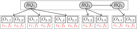
The HSP built for layer L1 is illustrated in Fig. 2. In the model, the root compound tasks are a set of observation requests Req, corresponding to areas of the field that must be observed. Each request RQj ∈ Req is decomposed into several (primitive) observation tasks made by Nj distinct robots, the idea being to build a schedule containing some redundancy to be robust to robot failures at execution time. Each request actually has several possible decompositions, corresponding to the candidate combinations of Nj distinct robots that can perform the corresponding observations. See the example of request RQ1, which can be realized through primitive observation tasks made by either {r1, r2}, or {r1, r3}, or {r2, r3}. The set of all primitive possible observation tasks is denoted by Obs, and each of these tasks has a fixed duration, together with release and due dates equal to 0 and H respectively, where H is the maximum duration of the mission.

Next, the model contains two kinds of resources, namely the set of robot resources Rob used to realize the observation tasks and the set of frequency resources F used to transfer observation data. Each primitive observation task simultaneously requires one robot resource and one frequency resource. All frequency resources are simple disjunctive resources (constant setup time equal to 0), while robots are disjunctive resources with setup times. For each robot r ∈ Rob and each pair of candidate observations (i, i′ ), setupr(i, i′ ) returns the duration required by r to move from the location of observation i to the location of observation i′ through the waypoint network. We extend setupr so that setupr(0, i′ ) gives the duration required to move from the initial location of r to observation i′ . In the set of constraints of the model, we also consider a set of acyclic precedence constraints P ⊆ Req × Req between requests. As explained previously, a CP model can be directly generated from the HSP illustrated in Fig. 2. Note that the problem solved in layer L1 is a kind of Sequence Dependent Setup Time Job Shop Scheduling Problem [Oddi et al., 2011].

6.4 Detailed SchedulingModel: Layer L2

Layer L2 is responsible for detailing the routing of robots and managing routing conflicts on the navigation graph. The latter is defined by a set of links L available between adjacent waypoints, and two robots cannot simultaneously use the same link. For L1, the set of resources to refine is the set of robots (Rref 1 = Rob), and for L2 the set of resources to consider is R2 = L∪F (the set of frequencies is kept in the set of resources since it is not refined by L2, i.e. F = R1\Rref 1 ).

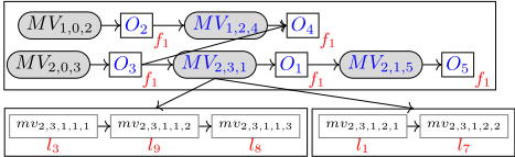
The HSP built for L2 is illustrated in Fig. 3, for an example involving two robots (requests RQj are not represented). The figure shows the sequence of high-level moves and observations realized by each robot in the solution σ1 produced by L1. In Fig. 3, the sequences of observations of robots are obsSeq1 = [2, 4] and obsSeq2 = [3, 1, 5]. Robot 1 must therefore realize a compound move MV1,0,2 from its initial location to observation number 2, then a primitive observation task O2, then a move MV1,2,4 from observation 2 to observation 4, and last a primitive observation task O4. Precedence constraints are imposed to guarantee that each robot realizes a move activity between two successive observations. The problem also contains precedence constraints between some observations (coming from the precedences required between observation requests). Each compound move MVr,i,i′ between two observations i, i′ is the root of a task network. It has as many decomposition methods as the number of possible paths between the location of i and the location of i′ (two possible decompositions in the case of compound move MV2,3,1). A decomposition using the pth path points to a task network which specifies a sequence of atomic moves mvr,i,i′ ,p,k required on links of the waypoint graph. Each atomic move consumes one link resource. For instance, the first path for MV2,3,1 traverses the sequence of links [l3, l9, l8], and each subtask mv2,3,1,1,k consumes the kth link of the sequence. Such a decomposition of moves between observations realized by each robot r is provided by the problem-specific function setupRefiner mentioned in Section 3. The setup operation setupOpr(i, i′ ) associated with each move from i to i′ for robot r corresponds to MVr,i,i′ in the example provided. As for layer L1, a CP encoding can be directly obtained from such a representation.

6.5 Experiments

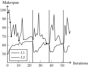
Instances. Experiments were performed over several multirobot problem instances generated randomly. These instances contain from 1 to 15 observation requests, each request requiring observations from 1 to 3 robots. From 1 to 3 frequencies are available to transfer observation data, and 3 robots are available to carry out the observations. Each robot has a different speed, which determines the duration needed to traverse a link. The field structure contains 3×|Req| waypoints connected to their closest neighbors within a fixed range. Function updateL1 is implemented with a learning rate α ranging from 0.2 to 1 and the reinitialization rate rateReinit for perturbL1 is 0.2. The scheduling problems were solved using IBM ILOG CP Optimizer 12.5 on an Intel Xeon E51603, 2.80GHz 8GB RAM, setting cpuMax = {5, 30} minutes and an adequate iterations number nLoops , depending on the number of observations (problem size) and the cpuMax . Interactions between layers L1/L2. To illustrate the interactions between the two layers, makespan results over iterations of the proposed approach are presented in Fig. 4 for a problem instance containing 5 observation requests (each one must be observed by 2 different robots). In order to accentuate the behavior, we have specifically implemented a very optimistic initL1 function to initialize setupr values to zero, using a learning rate α = 1. The best makespans successively obtained by L2 during the iterations are marked with a filled dot. Fig. 4 shows that makespans of both layers tend to converge quickly. When solutions cannot be improved, restarts are realized (vertical lines in the figure). More precisely, the first two restarts occurred when L1 did not find a solution better than the best one found so far, and the third restart when the makespan of the solution in L2 remained the same during several iterations. Since initL1 is very optimistic, the makespan of solutions of L1 tends to increase, given that values of coarse-grain setup times are also increasing.

Full Model. To compare the two-layer decision process with a global one-shot resolution strategy, we developed a global CP model. In theory, this model can be used to find an optimal solution. It contains (1) the model of layer L1 and (2) the model of layer L2 duplicated for each possible transition between observations. More precisely, it involves, for each robot r and each pair of distinct observations i, i′ , one optional taskMVr,i,i′ representing a global move of robot r from i to i′ , plus a huge number of optional intervals mvr,i,i′ ,p,k modeling the move of r on the kth link of the pth path available to go from i to i′ . The model contains a finegrain no overlap constraint that takes into account all observations and all move intervals over links, but to boost constraint propagation it also contains the coarse-grain no overlap constraint of layer L1 which takes into account all observation tasks and minimum setup times between them. Last, a constraint is added to ensure that the successive fine-grain activities realized by each robot have consistent types, i.e. that an observation interval associated with observation i is preceded by a move interval of the formMVr,i′ ,i.

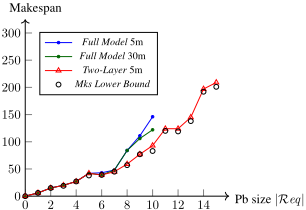
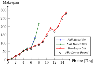
Comparison between the two-layer process and the Full Model. All generated instances have been solved using the two approaches. Representative results are given in Fig. 5 and 6, where the circle marks correspond to a makespan lower bound obtained from layer L1. For the instances of Fig. 5, only one robot must observe each request, and there are 0.2 × |Req|2 randomly generated precedences between requests. For Fig. 6, two distinct robots must observe each request and there are no precedences. Since the same makespan is reached for most of the experiments with several α values, we only present results for α = 0.7. Similarly, giving more CPU time to the two-layer process does not significantly improve the best solution, hence we only present the results for cpuMax = 5 minutes. For the Full Model, the generated instances contain from 14 tasks in the smallest instance to 139543 tasks in the largest one. For the largest instances, the Full Model does not find any solution, even with a CPU time of 30 minutes. The two-layer approach achieves better makespan results in a significantly shorter time, and the makespan values obtained are very close to the makespan lower bounds. It provides first solutions of good quality in less than 3 seconds (not represented on the figures), even for the largest instances in which the complete solver is not able to reach any solution after several minutes. For the smallest instances, the two-layer approach manages to find the optimal solution (without proving its optimality). These results demonstrate that the proposed iterative approach is both simple and much more effective than the Full Model for solving large-size instances. It allows to quickly get good quality solutions no matter the problem size, and intuitively the iterative process used allows L1 to propose very quickly different promising solutions to L2, based on approximations which can freely manipulate both lower and upper bounds on setup times, differently from approaches which would only manipulate valid cuts.

7 Conclusion

In this paper, we introduced techniques for scheduling with complex setup operations. As shown in the experiments, the approach exploits the strengths of existing CP solvers and gives acceptable computation times, even on problems for which the set of possible decompositions of setup operations is large. On the modeling side, we could add representation features to deal with task preconditions and task effects as in HTNs. On the algorithmic side, we could search for strategies that decompose compound tasks step-by-step, instead of having an arbitrary separation between two decision layers. Finally, decomposition structures allowing to derive efficient cuts for the layer L1 (LBBD) will be explored.