
Predict+Optimise with Ranking Objectives: Exhaustively Learning Linear Functions
Proceedings of the Twenty-Eighth International Joint Conference on Artificial Intelligence. Main track. Pages 1078-1085.
https://doi.org/10.24963/ijcai.2019/151
Keywords
- Constraints and SAT: Constraints and Data Mining ; Machine Learning
- Heuristic Search and Game Playing: Combinatorial Search and Optimisation
Abstract
We study the predict+optimise problem, where machine learning and combinatorial optimisation must interact to achieve a common goal. These problems are important when optimisation needs to be performed on input parameters that are not fully observed but must instead be estimated using machine learning. Our contributions are two-fold: 1) we provide theoretical insight into the properties and computational complexity of predict+optimise problems in general, and 2) develop a novel framework that, in contrast to related work, guarantees to compute the optimal parameters for a linear learning function given any ranking optimisation problem. We illustrate the applicability of our framework for the particular case of the unit-weighted knapsack predict+optimise problem and evaluate on benchmarks from the literature.
- [Azizi et al., 2018] Mohammad Javad Azizi, Phebe Vayanos, Bryan Wilder, Eric Rice, and Milind Tambe. Designing fair, efficient, and interpretable policies for prioritizing homeless youth for housing resources. In Integration of Constraint Programming, Artificial Intel- ligence, and Operations Research -15th International Conference, CPAIOR Proceedings, pages 35-51, 2018.
- [Berman et al., 2016] David Berman, Andre Cire, and Willian van Hoeve. Decisions diagrams for optimization. Springer, 2016.
- [Bessiere et al., 2017] Christian Bessiere, Frédéric Koriche, Nadjib Lazaar, and Barry O'Sullivan. Constraint acquisi- tion. Artificial Intelligence, 244:315 -342, 2017. Com- bining Constraint Solving with Mining and Learning. [Borchani et al., 2015]
- Hanen Borchani, Gherardo Varando, Concha Bielza, and Pedro Larrañaga. A survey on multi- output regression. Wiley Interdisciplinary Reviews: Data Mining and Knowledge Discovery, 5(5):216-233, 2015.
- [Demirović et al., 2019] Emir Demirović, Peter J. Stuckey, James Bailey, Jeffrey Chan, Chris Leckie, Kotagiri Ra- mamohanarao, and Tias Guns. An investigation into pre- diction + optimisation for the knapsack problem. In Inte- gration of Constraint Programming, Artificial Intelligence, and Operations Research -16th International Conference, CPAIOR, Proceedings, pages 241-257, 2019.
- [Donti et al., 2017] Priya L. Donti, Brandon Amos, and J. Zico Kolter. Task-based end-to-end model learning in stochastic optimization. In Proceedings of the 31st Con- ference on Neural Information Processing Systems (NIPS 2017), pages 5484-5494, 2017.
- [Dooren et al., 2017] David Van Den Dooren, Thomas Sys, Túlio A. M. Toffolo, Tony Wauters, and Greet Vanden Berghe. Multi-machine energy-aware scheduling. EURO J. Computational Optimization, 5(1-2):285-307, 2017.
- [Dragone et al., 2018] Paolo Dragone, Stefano Teso, and Andrea Passerini. Pyconstruct: Constraint programming meets structured prediction. In Proceedings of the Twenty- Seventh International Joint Conference on Artificial Intel- ligence, IJCAI-18, pages 5823-5825. International Joint Conferences on Artificial Intelligence Organization, 7 2018. IJCAI
- [Elmachtoub and Grigas, 2017] Adam N. Elmachtoub and Paul Grigas. Smart "predict, then optimize". Technical report, 2017. https://arxiv.org/pdf/1710.08005.pdf. Link
- [Gilmore and Gomory, 1966] PC Gilmore and Ralph E Go- mory. The theory and computation of knapsack functions. Operations Research, 14(6):1045-1074, 1966.
- [Grimes et al., 2014] Diarmuid Grimes, Georgiana Ifrim, Barry O'Sullivan, and Helmut Simonis. Analyzing the im- pact of electricity price forecasting on energy cost-aware scheduling. Sustainable Computing: Informatics and Sys- tems, 4(4):276-291, 2014. Special Issue on Energy Aware Resource Management and Scheduling (EARMS).
- [Joachims, 1998] Thorsten Joachims. Making large-scale svm learning practical. Technical report, Technical Report, SFB 475: Komplexitätsreduktion in Multivariaten Daten- strukturen, Universität Dortmund, 1998.
- [Joachims, 2002] Thorsten Joachims. Optimizing search engines using clickthrough data. In Proceedings of the Eighth ACM SIGKDD International Conference on Knowledge Discovery and Data Mining, KDD '02, pages 133-142. ACM, 2002.
- [Kotthoff, 2014] Lars Kotthoff. Algorithm selection for combinatorial search problems: A survey. AI Magazine, 35(3):48-60, 2014.
- [Liberto et al., 2016] Giovanni Di Liberto, Serdar Kadioglu, Kevin Leo, and Yuri Malitsky. DASH: dynamic approach for switching heuristics. European Journal of Operational Research, 248(3):943-953, 2016.
- [Lombardi et al., 2017] Michele Lombardi, Michela Milano, and Andrea Bartolini. Empirical decision model learning. Artificial Intelligence, 244:343-367, 2017.
- [Mathaba et al., 2014] Tebello Mathaba, Xiaohua Xia, and Jiangfeng Zhang. Analysing the economic benefit of elec- tricity price forecast in industrial load scheduling. Electric Power Systems Research, 116:158-165, 2014.
- [Passerini et al., 2017] Andrea Passerini, Guido Tack, and Tias Guns. Introduction to the special issue on combining constraint solving with mining and learning. Artif. Intell., 244:1-5, 2017.
- [Picard-Cantin et al., 2017] Émilie Picard-Cantin, Mathieu Bouchard, Claude-Guy Quimper, and Jason Sweeney. Learning the parameters of global constraints using branch-and-bound. In Principles and Practice of Con- straint Programming -23rd International Conference, CP 2017, Melbourne, VIC, Australia, August 28 -September 1, 2017, Proceedings, pages 512-528, 2017.
- [Pisinger and Røpke, 2010] David Pisinger and Stefan Røpke. Large neighborhood search. In Michel Gendreau and Jean-Yves Potvin, editors, Handbook of Metaheuris- tics, volume 146 of International Series in Operations Research & Management Science, chapter 13, pages 399-420. Springer, 2nd edition, 2010.
- [Teso et al., 2016] Stefano Teso, Andrea Passerini, and Paolo Viappiani. Constructive preference elicitation by setwise max-margin learning. In Proceedings of the Twenty-Fifth International Joint Conference on Artificial Intelligence, IJCAI, pages 2067-2073, 2016. IJCAI
- Wilder et al., ] Bryan Wilder, Bistra Dilkina, and Milind Tambe. Melding the data-decisions pipeline: Decision- focused learning for combinatorial optimization. In Pro- ceedings of the Thirty-Third AAAI Conference on Artificial Intelligence (AAAI-19).
- [Yue et al., 2007] Yisong Yue, Thomas Finley, Filip Radlin- ski, and Thorsten Joachims. A support vector method for optimizing average precision. In Proceedings of the 30th annual international ACM SIGIR conference on Research and development in information retrieval, pages 271-278. ACM, 2007.
References were extracted automatically from the PDF and may contain errors.
Full text extracted automatically from the PDF; figures, tables and equations may differ. The PDF is the version of record.
1 Introduction
As we are entering the age of automation with large data, there is an ever-growing need for the interpretability of the huge volume of available information as well as efficient resource utilisation. This requires two major research areas: machine learning and combinatorial optimisation. Advancement in these fields has resulted in many success stories and real-life applications over the last century. While a plethora of sophisticated algorithms and approaches are available in these fields respectively, an established methodology for solving problems which require both machine learning and combinatorial optimisation remains an open question.
Energy-aware scheduling [Mathaba et al., 2014; Grimes et al., 2014] is an example, where the goal is to schedule machines to perform tasks over a time period while minimising electricity costs. The electricity price, however, is not known upfront and must rather be estimated with machine learning based on weather forecasts. Therefore, optimisation needs to be performed with input that is not necessarily accurate.
Traditionally, the machine learning and combinatorial optimisation components are viewed as independent black-boxes: predict the input parameters and then optimise, hence the term predict+optimise [Demirovi´c et al., 2019]. The main issue that arises, however, is that conventional machine learning metrics, such as mean-square error, are not necessarily indicative for the outcome of the optimisation procedure.
Example 1. Consider a simplified project-funding problem. A limited number of projects can be selected and each results in a financial gain. There are two sets of estimates: P ′1 = (7, 6, 10) and P ′2 = (3, 10, 25), where the i-th component is the profit estimation of the i-th project pi. Let the true profits be given as P = (p1, p2, p3) = (5, 6, 10). Assume only two projects can be funded. Based on the estimates, the preferred choices are decision(P ′1 ) = {p1, p3} or decision(P ′2 ) = {p2, p3}. If the presented data was used in training a machine learning algorithm based on minimising mean-square error, i.e., mse(P ′ , P) = ∑j (p′j - pj)2 , estimate P ′1 would be deemed a more favorable prediction than estimate P ′2 as mse(P ′1 , P) = 4 < 245 = mse(P ′2 , P). However, in the context of optimisation, P ′2 yields a higher profit, i.e., P (decision(P ′1 )) = 15 < 16 = P (decision(P ′2 )).
Similar scenarios can be constructed with other standard metrics. Ideally, the optimisation result would be used as the machine learning metric, but as the combinatorial optimisation solutions are discrete, this gives rise to a nondifferentiable function. Hence, widely used techniques in machine learning, e.g., gradient descent, cannot be directly applied. This motivates the development of new machine learning algorithms that incorporate optimisation-problem knowledge.
Related work can be classified into three categories: 1) direct methods aim to interact with the optimisation problem during training by simplifying the setting, 2) semi-direct methods take into account features of the optimisation problem but do not directly interact during training, and 3) indirect methods are oblivious to the optimisation problem, i.e., standard machine learning algorithms such as linear regression. These approaches are discussed in more detail in Section 6.
Our contribution
In this work, we pose the following research questions:
- What are the properties and computational complexity of the predict+optimise problem?
- Can we design an algorithm that, based on the training sample, provably computes the optimal function for the predict+optimise setting?
- Can the computation be done efficiently in practice?
We address the first question by advancing the theoretical foundations of predict+optimise by characterising the properties and computational complexity in relation to the machine learning algorithm and optimisation problem. Individually, machine learning and optimisation are based on well-founded theories. However, such theories are not easily transferable to the predict+optimise setting and the interaction between the two components has yet to be understood. To obtain a deeper understanding of the interplay between machine learning and combinatorial optimisation, it is important to study the computational properties and limits from a theoretical side. Our results in Section 3 are a step in this direction.
The second research question is challenging as our theoretical results indicate that conventional techniques cannot be applied in a straight-forward fashion in general, unless P = NP. We tackle this question by providing a novel framework in Section 4 for the particular case where the machine learning component is a linear function and the combinatorial problem has a ranking objective, i.e., the optimisation outcome depends on the relative order of its input parameters and not their absolute values. The setting, even though restricted, covers an important class of problems in a theoretical and practical sense. Ranking problems appear in a variety of domains and some belong to the class of NP-hard problems, e.g., document retrieval [Joachims, 2002], houseallocation [Azizi et al., 2018], mean-average precision [Yue et al., 2007]. Linear functions are widely used in machine learning, e.g., regression and linear support vector machines.
There are three main advantages of our approach: it is an entirely new method for predict+optimise, which is generic for the considered problems, and complete, i.e., it can compute the optimal linear function given a training sample. Our framework admits any ranking optimisation problem, including NP-hard variants, and optimises with it directly, whereas in related work, challenging optimisation problems and/or resulting learning metrics are approximated with differentiable surrogates. Related work, in particular the relationship with preference elicitation, is discussed in Section 6.
The completeness aspect brings several benefits: it provides guarantees on the outcome and opens the possibility of new approximation methods that can directly use the optimisation problem as the learning metric. In addition, regularisation is included in our framework as a means to avoid overfitting. The flexible nature of our framework is paid in terms of computational time: it requires repeatedly solving the optimisation problem. Nevertheless, in Section 5, we demonstrate that our approach can be used in practice. To the best of our knowledge, our framework is the first of its kind for the predict+optimise setting.
2 Preliminaries
We define an optimisation problem as:
where P is the vector of optimisation parameters, C is the set of feasible solutions implicitly defined by a set of constraints, and obj is the objective function. Solving corresponds to computing an optimal solution X∗ that maximises the objective while respecting the constraints, i.e. X∗ ∈ {X|X ∈ C ∧ ∀X′ ∈ C : obj(X, P) ≥ obj(X′ , P)}.
Example 2 (continued). The simplified project-funding problem can be posed as obj(X, P) = ∑i Xi · pi and C = {X | ∀Xj , Xj ∈ {0, 1} ∧ ∑j Xj ≤ b}.
In the predict+optimise setting, the aim is to compute a solution X that maximises the objective in the optimisation problem, but the parameter vector P = (p1, p2, ..., pn) is hidden. To assist with the optimisation, a set of attribute vectors A are given, where Ai = (ai1, ai2, ..., aim) encodes partial information regarding the optimisation parameter pi.
Example 3 (continued Example 1). Each project pi is assigned an attribute vector Ai = (ai1, ai2), where ai1 and ai2 are integers denoting the experience of the project leader and market demand for project pi. The attribute vector Ai can assist in estimating the financial gain of project pi.
A common approach [Demirovi´c et al., 2019; Wilder et al., ; Elmachtoub and Grigas, 2017] is to take the solution obtained by solving the original optimisation problem using estimated parameters P ′ = f(A) rather than the hidden parameters P for a chosen function f . The predicted parameters P ′ are used to construct a solution, but its optimality is evaluated with respect to the hidden parameter P .
Example 4 (continued Example 1). Estimates P ′1 and P ′2 were used to compute decision(P ′1 ) and decision(P ′2 ), but only decision(P ′2 ) is optimal with respect to P .
The challenge is to select a function f that, when used to provide estimates, leads to an optimal solution with respect to the true parameters. Given historical data (Ai, pi), the aim is to compute f that minimises regret, i.e. the difference between the optimal solution and the resulting solution. Assume f belongs to a predetermined family of functions {fα} defined by their internal k-dimensional vector α. Therefore, the predict+optimise problem can be posed in terms of α:
The above equations represent the computation of α based on historical data (Ai, pi) during training. Afterwards, once an unknown instance consisting of attribute vectors A′i is given, the solution is determined using the calculated fα.
Similar definitions for this problem have appeared in literature, e.g. defining predict+optimise in terms of expected regret [Demirovi´c et al., 2019] and considering linear programs [Wilder et al., ; Elmachtoub and Grigas, 2017].
3 Properties of the Regret Function
We study the properties of Regret(α) (Equation 2) in terms of its two main components: the optimisation problem (obj,C) and the learning function fα. We characterise the co-domain of Regret(α), a sufficient condition for computing the optimal value, and its behaviour in each point in terms of discontinuity and gradient. This provides a basis for our approach. Intuitively, the results show the practical difficulty of predict+optimise.
Theorem 1. Regret(α) has finite co-domain if there exists a finite set of solutions Θ such that:
∀P ′ , ∀X∗ ∈ X∗ : obj(X∗ , P) ∈ {obj(X, P)|X ∈ Θ}, where X∗ = {X|X ∈ C ∧ ∀X′ ∈ C : obj(X, P ′ ) ≥ obj(X′ , P ′ )}.
The proof is by contradiction. The main step is to prove the existence of Θ for a particular predict+optimise setting.
Corollary 1. Regret(α) has finite co-domain if:
- the optimisation problem has a finite co-domain; or
- the set of feasible solutions |C| is finite; or
- the optimisation problem is a linear program, i.e. it can be posed as: maxX(cT X) s.t. AX ≤ b.
Proof. The first case is straight-forward, while the second follows as it is sufficient to set Θ = C. For the third case, it is known in linear programming theory that if there exists a feasible solution, then there exists an optimal solution in an extremal point of the polyhedron defined by the linear constraints. Let Θ be the set of all extremal points. It follows that Θ is finite and given an arbitrary P, each optimal solution will be covered by at least one solution in Θ.
Remark 1. According to Theorem 1, even though the sets of feasible and optimal solutions are uncountable for linear programs in general, Regret(α) has a finite co-domain.
Theorem 1 gives rise to the following key theorem, which makes a statement about optimality search:
Remark 2. For Regret(α) with finite co-domain, it is sufficient to evaluate a finite number of points ζ in the parameter space to compute the optimal α that minimises regret, even if the domain of Regret(α) is continuous.
Note that the previous theorem only asserts the existence of ζ, but does not provide explicit guidance for its computation. This is discussed in the next section for a special case.
Theorem 2. If Regret(α) has finite co-domain, then given a point α′ , exactly one of the following holds:
- the gradient in α′ is zero, i.e. ∇Regret(α′ ) = 0.
- α′ is a point of discontinuity of Regret(α).
Remark 3. If Regret(α) has finite co-domain, its set of nondifferentiable points is infinite in general.
Theorem 2 and Remark 3 provide an intuitive explanation for the difficulty of solving predict+optimise in practice: the resulting regret function that needs to be optimised is typically nonlinear, nondifferentiable, and has gradient zero in its continuous points. Therefore, for instance, widely used gradient descent methods cannot be directly applied.
Remark 4. The previous remarks and propositions hold in general regardless of the characterisation of fα.
3.1 Computational Complexity
We show the theoretical limitations of predict+optimise. The results indicate that conventional techniques are unlikely to provide satisfactory solutions. Intuitively, predict+optimise is more difficult than each of its individual components, which in turn motivates the development of novel approaches.
Definition 1. (Decision Problem for Regret - DPR)
- Input: Rational number c, regret function Regret(α) with an internal learning function fα
- Question: Does there exist α such that Regret(α) ≤ c?
Definition 2. opt(P) = argmaxX∈C{obj(X, P)}.
Proposition 1. DPR is in the class NP if both fα and opt(P ) can be evaluated in polynomial time.
Note that evaluating fα and opt(P) is sufficient to answer the decision problem given a particular value α.
Proposition 2. DPR is NP-hard if fα or opt(P) is NPhard.
Informally speaking, the proof follows since solving the NP-hard problem is part of computing the regret function.
Corollary 2. NP-completeness of DPR implies P = NP.
The corollary follows from the definition of NP-hardness. In particular, Corollary 2 illustrates that, unless NP = P, we cannot in general answer DPR by reducing it to standard NPcomplete combinatorial frameworks, such as the satisfiability problem (SAT) or integer programming.
4 Framework for Predict+Optimise
We provide a novel approach to compute α∗ that minimises Regret(α) for the following predict+optimise setting:
- The ranking property is satisfied (Definition 5).
- fα is linear, i.e. fα(Ai) = α · Ai for α ∈ Rn .
The advantage of our method is that we directly optimise using the regret function in a complete fashion and therefore guarantee to find the global minimum α∗ . We divide this section into three subsections: 1) Core - the main results, 2) Extension - extends the results for the case where multiple optimisation instances must be optimised with the same α, corresponding to a training set in machine learning with more than one optimisation benchmark, and 3) Computational enhancements - important techniques for practical computation.
4.1 Core
We introduce the class of problems considered and an algorithm for the optimal α∗ of Regret(α) for these problems.
We give two definitions prior to the ranking property, which characterises the optimisation problems covered.
Definition 3. TP(P) is the total preorder defined by P, i.e. TP(P) = {(i, j) | i, j ∈ {1, 2, ..., dim(P)} ∧ pi ≥ pj}, where dim(P) is the dimension of the parameter vector P.
Definition 4. optSols(P) = {X∗ | X∗ ∈ C ∧ ∀X′ ∈ C : obj(X∗ , P ) ≥ obj(X′ , P )}.
Definition 5 (Ranking property). An optimisation problem (obj(X, P),C) satisfies the ranking property if: ∀P1, P2 : TP(P1) = TP(P2) =⇒ optSols(P1) = optSols(P2).
Example 5 (continued Example 2). The simplified projectfunding problem satisfies the ranking property. Consider parameter vectors P1 = (50, 15, 25) and P2 = (3, 1, 2). Both result in the same total preorder, i.e. TP = {(p1, p2), (p1, p3), (p3, p2)}, and hence lead to the same optimal solution {p1, p3} for b = 2.
We label the resulting regret function as Regretrank lin (α) to differentiate it from the general case. The ranking property is imposed as it represents a meaningful subclass of problems with an exploitable structure which are practically relevant e.g. document retrieval [Joachims, 2002] and youth-house allocation [Azizi et al., 2018].
Proposition 3. The objective function of an optimisation problem satisfying the ranking property has finite co-domain.
Corollary 3. Regretrank lin (α) has finite co-domain.
The aim is to compute α that minimises Regretrank lin (α). Corollary 3 implies Remark 2, and thus it is sufficient to compute the finite set of points ζ from Remark 2 and evaluate each point to obtain the minimising α∗ .
In the following, we provide an algorithm that computes a finite set of points ζ s that is guaranteed to be a superset of the key points, i.e. ζ ⊆ ζ s .
Remark 5. The function fα defines a total preorder over the optimisation parameters P and attribute vectors Ai.
Definition 6. (change in ranking) Given α1 and α2 , optimisation parameters pi and pj with corresponding attribute vectors Ai and Aj, we say that there is a change in ranking from α1 to α2 for pi and pj (and consequently for Ai and Aj) if fα1(Ai) ◦1 fα1(Aj) ∧ fα2(Ai) ◦2 fα2(Aj) for (◦1, ◦2) = (<, >) or (◦1, ◦2) = (>, <).
Proposition 4. The domain of Regretrank lin (α) can be reduced to a finite set.
This is consistent with Remark 2. The remaining challenge is to efficiently calculate the reduced domain. A key ingredient is given in the following theorem.
Proposition 5. For α1 and α2 such that Regretrank lin (α1 ) ̸= Regretrank lin (α2 ), there exist two optimisation parameters for which there is a change in ranking from α1 to α2 .
Remark 6. A change in ordering is not a sufficient condition for a change in regret in general.
According to Proposition 5, we conclude it is sufficient to restrict the domain of Regretrank lin (α) to the set of points that are infinitesimally close to the points where pair-wise optimisation parameters pi and pj are considered equivalent with respect to the total preorder defined by f, i.e. domain = ⋃i,j {t | fα(Ai) = fα(Aj) ∧ |α - t| ≤ ϵ} for some small ϵ ≥ 0. We label these values as transition points, as a change in regret can only occure in their small neighbourhood.
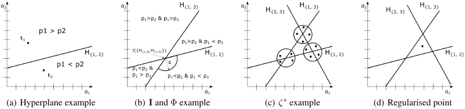
Example 6. Figure 1(a) shows the transition points for two parameters p1 and p2 and a vector α = (α1, α2) of two dimensions. The line represents the transition points. The relative ranking of the parameters p1 and p2 only changes in the neighbourhood of the transition points. Consecutively, Proposition 5 and Remark 6 state that considering the close neighbourhoods of transition points does not remove all optimal α∗ which minimise regret.
However, the resulting set of points is infinite for a vector α with more than one dimension. Therefore, further filtering is required to obtain the finite set of points ζ from Remark 2. Before presenting the main theorem for computing the finite set, we first provide several definitions. Furthermore, to ease the understanding of the approximation in Section 4.3, without loss of generality, assume that f adds a constant ci to each prediction depending on the optimisation parameter pi.
Definition 7. H{i,j} is the hyperplane where the parameters i and j have equal rank according to fα, i.e. for i ̸= j, H{i,j} = {α | fα(Ai) = fα(Aj)}.
Example 7. Figure 1(a) shows a 2D hyperplane H{1,2} for α = (α1, α2) where p1 = p2. Each hyperplane separates the space into two regions: all points above and below H{1,2} define an ordering with p1 > p2 and p1 < p2, respectively.
Definition 8. Let dim(P) = n. H∗ is the set containing all H{i,j}, i.e. H∗ = {H{i,j} | i, j ∈ {1, 2, ..., n} ∧ i ̸= j}.
Definition 9. H|α| is the set of sets of H{i,j} with cardinality dim(α), i.e. H|α| = {K | K ⊆ H∗ ∧ |K| = dim(α)}.
Definition 10. Let rand(S) be the function that arbitrary selects a point from the set S.
Definition 11. I(K) for K ∈ H|α| is the set of intersection points of hyperplanes H{i,j} ∈ K, i.e. ⋂H{i,j}∈K H{i,j}.
Definition 12. Let order(S) be the set of total preorderings of elements from S.
Example 8. Let order({a, b}) = {{(a, b)}, {(b, a)}, {(a, b), (b, a)}}. The pairs (a, a) and (b, b) present in each total preorder omitted for clarity. The first two preorders define strict orderings, while elements are considered equal in the last case.
Definition 13. Φ(E, α, ord) is the set of points infinitesimally close to α for which ft∈Φ respects the order defined in ord for elements in E, i.e. Φ(E, α, ord) = {t : |α- t| ≤ ϵ ∧ ft =⇒ (∀i, j ∈ E, i ̸= j : ft(Ai) ⪯ ft(Aj) → (i, j) ∈ ord)} for some small ϵ ≥ 0.
Example 9. Figure 1(b) shows the intersection point I({H{1,2},H{1,3}}). Φ(G, I, {(p1 < p2), (p1 < p3)}) consists of every point in between the arc of radius ϵ and the two hyperplanes, while G would be the circle containing the arc (G not shown in image). Note that each of the four areas around the intersection define a different ordering.
Definition 14. σ(K) is the set of indices that were used in defining the dim(α)-tuple K, i.e. σ(K) = {i | H{i,j} ∈ K}.
Definition 15. Ekn is the set of subsets of {1, 2, ..., n} with cardinality k, i.e. Ekn = {e | e ⊆ {1, 2, ..., n} ∧ |e| = k}.
Assume the hyperplanes H{i,j} are nonparallel and |H∗ | ≥ dim(α). We may now state the main definition and theorem. Definition 16. ζ s is the set of points infinitesimally close to all possible dim(α)-hyperplane intersections that locally define unique rankings of attribute vectors, i.e. ζ s = {rand(Φ(σ(K), rand(IK), ord)) | K ∈ H|α| ∧ ord ∈ order(σ(K)) ∧ Φ(σ(K), rand(IK), ord) ̸= {∅}}.
Example 10. Figure 1(c) shows ζ s for a problem with three optimisation parameters. The set ζ s consists of 12 points, each located within ϵ distance from an intersection point.
Theorem 3. ζ s is a superset of ζ from Rm. 2, i.e. ζ ⊆ ζ s .
Corollary 4. The optimal α∗ = argminαRegretrank lin (α) can be computed by evaluating each point in ζ s .
Proof of Th. 3 follows from Lemmas 1 and 2 given below.
Lemma 1. For each α ∈ R, there exists α′ ∈ ζ s such that Regretrank lin (α) = Regretrank lin (α′ ).
Lemma 2. ζ s may contain redundant points, i.e. points that map to the same co-domain.
The redundant points from Lemma 2 are partially due to Remark 6. A subset of the points from ζ s induce changes in the ranking of the optimisation parameters that do not have an effect on the final solution.
Theorem 3 and ζ s provides the key points among which is at least one point that minimises the regret. Thus, evaluating each point from ζ s leads to the computation of the optimal α.
Remark 7. The set of optimal points is uncountable for continuous fα. In particular, the points are given by the polyhedron enclosed by the neighbouring Hi,j .
Example 11. Let α∗ be the middle point in Figure 1(d). Each point on the polygon is an optimal point.
4.2 Extension
In real-life scenarios, the input data might contain multiple instances of the optimisation problem where learning α is done across all problems. The previous results can be generalised for this case. Formally, the setting is analogous to before, but the input consists n benchmarks, i.e. n sets of Pi, Ai, and Ci. Regret is extended as the sum of the regret of individual benchmarks, i.e. Regret(α) = ∑i Regreti(α) = ∑i (obj(X∗ i , Pi) - obj(Xi(α)′ , Pi)). The goal is, as before, to compute a single α to minimise the regret. Note that if n = 1, we obtain the previously discussed setting.
Example 12. In the simplified project-funding problem, one might consider historical data of the past ten years. In this setting, assuming the funding decisions are made annually, the task is to compute a learning function that leads to minimum regret when considering the sum of regrets of each individual year, where the regret of each year is represented by an instance of the project-funding problem from Example 2.
We now extend the definition of the main set, ζ s .
Proposition 6. Given n benchmarks, the extended ζ s ext can be computed as the union of the individual ζ s i , i.e. ζ s ext = ∪iζ s i , where ζ s i is the ζ s from Thm. 3 for the i-th benchmark.
Proof. Let α∗ = argminα∈ζ s ext Regretrank lin (α) and assume ∃α′ : Regretrank lin (α′ ) < Regretrank lin (α∗ ) and therefore α′ ̸∈ ζ s ext . It follows from Prop. 5 that there must be a change in ranking from α∗ to α′ for at least one benchmark, implying ∃α′′ ∈ ζ s ext : fα′ = fα′′ . Thus, Regretrank lin (α∗ ) ≤ Regretrank lin (α′′ ), but by assumption we have Regretrank lin (α′ ) < Regretrank lin (α∗ ) which is a contradition as Regretrank lin (α′ ) = Regretrank lin (α′′ ).
4.3 Computational Enhancements
We provide techniques to reduce the number of points in ζ s , which naturally provides speed-ups in practice. In addition, we discuss an approximation of our approach, offering a trade-off between computational time and optimality.
Filtering based on the preorder. Lemma 2 consequently offers insight for practical computation. Speed-ups could be obtained by discarding a point that defines the same total preordering as a previously computed point.
Filtering based on objective. Motivated by Remark 6, given an α′ , we may filter the set H|α| based on the contribution of the correct ordering of the optimisation parameters.
Definition 17. Let F ∗ = {f | argminf Regret(f)|}.
Definition 18. Let rank(Ai, f) be the rank of the i-th optimisation parameter induces by the total preorder of f.
Definition 19. Given an fα, the i-th optimisation parameter is violating in fα if ∄f ∈ F ∗ : rank(Ai, fα) = rank(Ai, f).
Proposition 7. Given fα′ , we may remove K from H|α| without losing optimality if σ(K) does not contain any violating optimisation parameter in fα′ .
Exploiting Proposition 7 requires efficiently testing if a parameter is violating, which depends on the optimisation problem. This can be done for the project-funding problem.
Filtering based on multiple benchmarks. The regret of the individual benchmark can be used as an additional filter:
Proposition 8. For α ∈ ζ s ext , we can remove every α′i ∈ ζ s i from ζ s ext such that Regreti(α′i ) > Regreti(α) without removing all α∗ = arg minα′′∈ζ s ext Regretrank lin (α′′ ) from ζ s ext .
Regularisation. In the previous text, we considered points infinitesimally close to an intersection. To account for overfitting, we may consider the centroid point of the polyhedron enclosed by neighbouring Hi,j which contains the infinitesimally close point, as regret is constant along the polyhedron.
Example 13. Let the three points in the middle polygon in Figure 1(c) be optimal points. The centroid point displayed in Figure 1(d) is the regularised point.
Approximation - Large Neighbourhood Search (LNS). Given an initial αinit = (α1, α2, ..., ...αn), we proceed with our approach as before but fix a subset of the coefficients to their current values in αinit, effectively treating them as constants. This reduces the search and any solution that improves the regret for the reduced problem does so for the original problem as well. The procedure can be repeated iteratively with different subsets of the coefficients until a specified timeout is reached, providing a trade-off between optimality and computational time. This resembles large neighbourhood search [Pisinger and Røpke, 2010] from the meta-heuristic community, but applied to parameters of the regret function.
5 Experimental Results
The goal is to provide a proof-of-concept implementation that illustrates the effectiveness of our approach in practice. We provide two sets of experiments. The first demonstrates the computational benefits of techniques from Section 4.3. The second compares our approach with the state-of-the-art.
5.1 Benchmarks and Data
We experiment with artificial and real-life energy-price datasets as used in [Demirovi´c et al., 2019] with the unitweighted knapsack predict+optimise problem [Gilmore and Gomory, 1966], which corresponds to the project-funding problem introduced in the examples.
The artificial dataset was constructed such that the profits cannot be easily learned: the tuples (pk,Ak) are generated as pk = 103 sin(i)sin(j) and Ak = (i, j), and partitioned into benchmarks. The profits are further multiplied by a different constant for each benchmark. The dataset contains 1000 benchmarks and 48 optimisation parameters per benchmark.
The real-life datasets contain two years of historical energy price data from the day-ahead market of SEM-O, the Irish Single Electricity Market Operator. The data was used in the ICON energy-aware scheduling competition and a number of publications, e.g. [Grimes et al., 2014; Dooren et al., 2017]. The attributes consist of the date of the day, weather information, e.g. estimates of the temperature, wind speed, and CO2 intensity in Cork, and lastly the price predictions given by the energy company. Note that predictions are not made from scratch, but rather based on predictions of the company together and weather information. Each benchmark represents a day and each optimisation parameter represents the price for one half-hour. The dataset contains 37,872 benchmarks, 48 optimisation parameters per benchmark, and the attribute vectors are compressed to eight features.
5.2 LearningMethods andMethodology
We compare with the state-of-the-art techniques for predict+optimise detailed in Section 6. (Indirect) Ridge regression; SVMR; (direct) SPO, smart predict then optimise [Elmachtoub and Grigas, 2017]; (semi-direct) QPTL-s, quadratic programming task loss [Wilder et al., ] specific to the knapsack problem [Demirovi´c et al., 2019]; and SVM-s, learn-topartition[Demirovi´c et al., 2019]. Multi-output ridge regression [Borchani et al., 2015] was not used as it was dominated by its single output variant.
Training and test sets are divided at a 70%-30% ratio. Our approach solves the artificial dataset optimally and uses LNS from Section 4.3 for the energy dataset, optimising one parameter at a time. Initial coefficients were based on SVM-s. For other methods, we performed 5-fold hyperparameter tuning with regret as the measure.
5.3 Effect of Techniques from Section 4.3
We run our algorithm for the energy-pricing dataset with different combinations of techniques. The capacity was set to 10% of total number of optimisation parameters, i.e. b = 4 in Example 2. In Table 1, each row shows the runtime and number of points fully evaluated followed by entries indicating which technique was used. The baseline is given in the last row. Using multiple benchmark- and objective-based filtering individually provides a substantial reduction in time as they both avoid fully evaluating a large number of points. Multiple benchmark filtering is stronger, i.e. produces fewer points, albeit more computationally demanding when compared to objective-based filtering, and hence the runtime difference. Combining both techniques leads to better results. Further including preorder filtering discards additional points. The best variant is composed of all three techniques, and achieves an order-of-magnitude improvement in terms of runtime and points evaluated over the baseline.
5.4 Comparison with the state-of-the-art
We discuss both datasets by setting the capacity b to 10%, 30%, and 50% of the number of optimisation parameters. In Table 2, entries (x, y) represent the average regret for the training (x) and testing set (y). The values are in thousands for the artificial dataset.
Our approach, labelled LinRankOpt, computes the optimal coefficients for the artificial dataset. Thus, on the training set, it achieves the minimum regret and provides the best results when compared to other techniques. The exception is SVMs, which obtains the best results as well. Small differences can be observed in the test set due to different regularisation policies. In addition, our approach was able to provide slight improvements over the baseline SVM-s for the energy dataset.
| Techniques from Section 4.3 | ||||
|---|---|---|---|---|
| Runtime (s) | # points | preorder | objective | multi-bench |
| 129 | 1k | 1 | 1 | 1 |
| 140 | 1.2k | 0 | 1 | 1 |
| 259 | 2.2k | 0 | 1 | 0 |
| 351 | 1.7k | 0 | 0 | 1 |
| 2152 | 18k | 0 | 0 | 0 |
| Indirect | Semi-direct | Direct | ||||
|---|---|---|---|---|---|---|
| Capacity | ridge | SVMR | QPTL-s | SVM-s | SPO | LinRankOpt |
| Artificial Dataset | ||||||
| 5 (10%) 15 (30%) 25 | (12.0; 12.0) | (1.12; 0.99) | (24.22; 23.68) | (0.08; 0.41) (0.5; 0.27) | (20.49; 20.36) | (0.07; 0.09) (0.25; 0.032) |
| (11.0; 12.0) | (2.29; 2.54) | (35.34; 34.76) | (30.31; 29.75) | |||
| (50%) | (1.1; 0.9) | (4.71; 6.07) | (0.1; 0.0) | (0.04; 0.03) | (0.38; 0.13) | (0.03; 0.06) |
| Energy-Pricing Dataset | ||||||
| 5 (10%) | (43; 51) | (39; 44) | (50; 64) | (41; 42) | (40; 55) | (39; 44) |
| 15 (30%) | (59; 67) | (55; 53) | (76; 105) | (55; 51) | (59; 72) | (53; 51) |
| 25 (50%) | (42; 48) | (38; 41) | (49; 70) | (39; 45) | (36; 45) | (37; 40) |
The experimentation illustrates the practicality of our novel method: it achieves better or comparable results to the stateof-the-art for the two datasets. Its advantage is that it can directly optimise the linear function with respect to the ranking combinatorial problem. The drawback is that, at its current state, the runtime can be longer than the other approaches, as it involves repeatedly solving the optimisation problem. Nevertheless, the runtime in experiments was within minutes.
6 RelatedWork
6.1 Predict+optimise
Previous approaches for predict+optimise can be partitioned into three groups. Indirect methods use standard learning methods and loss functions that are independent of the optimisation problem. Two algorithms in this category have been applied in [Demirovi´c et al., 2019]: linear regression and SVMRank [Joachims, 2002; Joachims, 1998]. Both compute a value for an optimisation parameter as a linear combination of its attributes with different goals: linear regression optimises to capture the precise value of the parameter, while SVMRank computes the relative ranking between parameters.
Semi-direct methods [Demirovi´c et al., 2019] take into account the optimisation problem, but in an indirect fashion. For example, a learning algorithm may learn to classify items in knapsack problems as desirable and not desirable. This approach may offer advantages over pure ranking approaches.
Direct methods [Wilder et al., ; Elmachtoub and Grigas, 2017] interact with the optimisation problem during training. For convex quadratic programs, the gradient of argmax can be computed [Donti et al., 2017]. For combinatorial problems, convex surrogates are employed in training through gradient descent techniques of proxy problems, thus simplify the problem and not consider it directly. It is not trivial to incorporate combinatorial problem in the learning metric, as it leads to a nondifferentiable metric function. This is a critical difference in our approach, where we provide means of directly optimising the learning algorithm with the optimisation problem.
6.2 Other related approaches
Our approach falls into the broad research theme of combining machine learning and constraint optimisation [Passerini et al., 2017]. Most research has focussed on using machine learning to improve the solving process, e.g. algorithm selection and hyperparameter optimisation [Kotthoff, 2014] and using machine learning to improve mixed-integer programming solvers [Liberto et al., 2016]. This differs from our setting, where the aim is to develop machine learning algorithms designed to learn input parameters of a combinatorial optimisation problems are estimated with machine learning rather than given precisely. Optimisation and machine learning are necessary to solve predict+optimise rather than having machine learning to boost the optimisation process.
In terms of modelling, constraint acquisition [Bessiere et al., 2017] uses machine learning techniques to learn structural constraints from data, while other works are concerned with finding the most likely parameters of given hard constraints [Picard-Cantin et al., 2017].
The emerging topic of constructive machine learning and preference elicitation [Dragone et al., 2018; Teso et al., 2016] is closely related, where the goal is to learn to synthesize structured objects from data, e.g. interactively learning the preferences of a user and searching for the most preferred object. Our setting bears several similarities with preference elicitation, e.g. both frameworks aim to learn a linear function with unknown parameters whilst minimising a related notion of regret. Solutions and weights in preference elicitation correspond to attribute vectors and α. However, there are notable differences. Incremental preference elicitation considers querying the user, uses a single optimisation problem, and considers pairwise comparisons with additional constraints. In contrast, our setting assumes a fixed dataset, simultaneously optimises multiple problems with the same α, use a test set in addition to a training set, and our ranking property allows capturing certain nonlinear relationships between input data. In both settings, the predictions are used in the objective, but our work is concerned with learning the weights of the objective on a per-instance basis.
Two-phase approaches, which view the machine learning and optimisation component as independent black-boxes, were used in energy-aware load shifting [Mathaba et al., 2014; Grimes et al., 2014]. In addition, it has been applied in a setting where the objective function is learned based on data extracted from simulations [Lombardi et al., 2017]. The learnt function is afterwards embedded into a declarative statement of the optimisation problem. The approach can be seen as indirect with the main challenge of gathering representative training data from a simulation and analysing the feasibility of embedding machine learning approaches into the declarative statement of the optimisation problem.
7 Conclusion
We presented theoretical insights into the predict+optimise problem and a novel framework that can learn linear functions by directly interacting with the underlying combinatorial ranking optimisation problem. There are several main directions for future work: 1) an extension for arbitrary optimisation problems, which seems challenging but Theorem 1 indicates that it is possible, 2) improve the anytime performance, and 3) knowledge compilation [Berman et al., 2016] which may speed-up resolving the optimisation problem.
@inproceedings{ijcai2019p151,
  title     = {Predict+Optimise with Ranking Objectives: Exhaustively Learning Linear Functions},
  author    = {Demirović, Emir and Stuckey, Peter J. and Bailey, James and Chan, Jeffrey and Leckie, Christopher and Ramamohanarao, Kotagiri and Guns, Tias},
  booktitle = {Proceedings of the Twenty-Eighth International Joint Conference on
               Artificial Intelligence, {IJCAI-19}},
  publisher = {International Joint Conferences on Artificial Intelligence Organization},
  editor    = {Sarit Kraus},
  pages     = {1078--1085},
  year      = {2019},
  month     = {8},
  note      = {Main track},
  doi       = {10.24963/ijcai.2019/151},
  url       = {https://doi.org/10.24963/ijcai.2019/151},
}
TY - CPAPER TI - Predict+Optimise with Ranking Objectives: Exhaustively Learning Linear Functions AU - Demirović, Emir AU - Stuckey, Peter J. AU - Bailey, James AU - Chan, Jeffrey AU - Leckie, Christopher AU - Ramamohanarao, Kotagiri AU - Guns, Tias T2 - Proceedings of the Twenty-Eighth International Joint Conference on Artificial Intelligence, IJCAI-19 PB - International Joint Conferences on Artificial Intelligence Organization PY - 2019 SP - 1078 EP - 1085 DO - 10.24963/ijcai.2019/151 UR - https://doi.org/10.24963/ijcai.2019/151 ER -Copied
Machine-readable versions of this paper, for tools and AI agents:





