
Constraint Programming for Mining Borders of Frequent Itemsets
Proceedings of the Twenty-Eighth International Joint Conference on Artificial Intelligence. Main track. Pages 1064-1070.
https://doi.org/10.24963/ijcai.2019/149
© 2019 International Joint Conferences on Artificial Intelligence
Keywords
- Constraints and SAT: Global Constraints
Abstract
Frequent itemset mining is one of the most studied tasks in knowledge discovery. It is often reduced to mining the positive border of frequent itemsets, i.e. maximal frequent itemsets. Infrequent itemset mining, on the other hand, can be reduced to mining the negative border, i.e. minimal infrequent itemsets. We propose a generic framework based on constraint programming to mine both borders of frequent itemsets.One can easily decide which border to mine by setting a simple parameter. For this, we introduce two new global constraints, FREQUENTSUBS and INFREQUENTSUPERS, with complete polynomial propagators. We then consider the problem of mining borders with additional constraints. We prove that this problem is coNP-hard, ruling out the hope for the existence of a single CSP solving this problem (unless coNP ⊆ NP).
- [Adda et al., 2007] M. Adda, L. Wu, and Y. Feng. Rare itemset mining. In Proceedings of ICMLA'07, Cincinnati, Ohio, USA, pages 73-80. IEEE, 2007.
- [Agrawal and Srikant, 1995] R. Agrawal and R. Srikant. Mining sequential patterns. In Proceedings of ICDE'95, Taipei, Taiwan, pages 3-14. IEEE, 1995.
- [Agrawal et al., 1994] R. Agrawal, R. Srikant, et al. Fast al- gorithms for mining association rules. In Proceedings of VLDB'94, Santigo de Chile, Chile, volume 1215, pages 487-499, 1994.
- [Bastide et al., 2000] Y. Bastide, R. Taouil, N. Pasquier, G. Stumme, and L. Lakhal. Mining frequent patterns with counting inference. ACM SIGKDD Explorations Newslet- ter, 2(2):66-75, 2000.
- [Belaid et al., 2019] M.B. Belaid, C. Bessiere, and N. Lazaar. Constraint programming for association rules. In Proceedings of SDM'19, Calgary, Alberta, Canada. SIAM, 2019.
- [Berge, 1984] C. Berge. Hypergraphs: combinatorics of fi- nite sets, volume 45. Elsevier, 1984.
- [Bessiere et al., 2018] C. Bessiere, N. Lazaar, and M. Maa- mar. User's constraints in itemset mining. In Proceedings of CP'18, Lille, France, pages 537-553. Springer, 2018.
- [Bonchi and Lucchese, 2004] F. Bonchi and C. Lucchese. On closed constrained frequent pattern mining. In Pro- ceedings of ICDM'04, Brighton, UK, pages 35-42. IEEE, 2004.
- [Boros et al., 2003] E. Boros, V. Gurvich, L. Khachiyan, and K. Makino. On maximal frequent and minimal infrequent sets in binary matrices. Annals of Mathematics and Artifi- cial Intelligence, 39(3):211-221, 2003.
- [Burdick et al., 2001] D. Burdick, M. Calimlim, and J. Gehrke. Mafia: A maximal frequent itemset algorithm for transactional databases. In Proceedings of ICDE'01, Heidelberg, Germany, pages 443-452. IEEE, 2001.
- [De Raedt et al., 2008] L. De Raedt, T. Guns, and S. Nijssen. Constraint programming for itemset mining. In Proceed- ings of KDD'08, Las Vegas, Nevada, USA, pages 204-212. ACM, 2008.
- [Dong and Li, 1999] G. Dong and J. Li. Efficient mining of emerging patterns: Discovering trends and differences. In Proceedings of KDD'99, San Diego, California, USA, pages 43-52. Citeseer, 1999.
- [Gouda and Zaki, 2001] K. Gouda and M.J. Zaki. Efficiently mining maximal frequent itemsets. In Proceedings of ICDM'01, San Jose, California, USA, page 163. IEEE, 2001.
- [Grahne and Zhu, 2003] G. Grahne and J. Zhu. Efficiently using prefix-trees in mining frequent itemsets. In Proceed- ings of FIMI'03, Melbourne, Florida, USA, volume 90, 2003.
- [Haglin and Manning, 2007] D.J. Haglin and Anna M. Man- ning. On minimal infrequent itemset mining. In Proceed- ings of DMIN'07, Las Vegas, Nevada, USA, pages 141- 147, 2007.
- [Han et al., 2000] J. Han, J. Pei, and Y. Yin. Mining frequent patterns without candidate generation. In ACM sigmod record, volume 29, pages 1-12. ACM, 2000.
- [Khiari et al., 2010] M. Khiari, P. Boizumault, and B. Crémilleux. Constraint programming for mining n-ary patterns. In Proceedings of CP'10, St Andrews, Scotland, pages 552-567. Springer, 2010.
- [Lazaar et al., 2016] N. Lazaar, Y. Lebbah, S. Loudni, M. Maamar, V. Lemière, C. Bessiere, and P. Boizumault. A global constraint for closed frequent pattern mining. In Proceedings of CP'16, Toulouse, France, pages 333-349. Springer, 2016.
- [Liu et al., 1999] B. Liu, W. Hsu, and Y. Ma. Mining as- sociation rules with multiple minimum supports. In Pro- ceedings of KDD'99, San Diego, California, USA, pages 337-341. ACM, 1999.
- [Mannila and Toivonen, 1997] H. Mannila and H. Toivonen. Levelwise search and borders of theories in knowledge dis- covery. Data mining and knowledge discovery, 1(3):241- 258, 1997.
- [Negrevergne et al., 2013] B. Negrevergne, A. Dries, T. Guns, and S. Nijssen. Dominance programming for itemset mining. In Proceedings of ICDM'13, Dallas, Texas, USA, pages 557-566. IEEE, 2013.
- [Nourine and Petit, 2012] L. Nourine and J.M. Petit. Extend- ing set-based dualization: Application to pattern mining. In Proceedings of ECAI'12, Montpellier, France, pages 630-635. IOS Press, 2012.
- [Pasquier et al., 1999] N. Pasquier, Y. Bastide, R. Taouil, and L. Lakhal. Discovering frequent closed itemsets for associ- ation rules. In Proceedings of ICDT'99, Jerusalem, Israel, pages 398-416. Springer, 1999.
- [Rossi et al., 2006] F. Rossi, P. Van Beek, and T. Walsh. Handbook of constraint programming. Elsevier, 2006.
- [Schaus et al., 2017] P. Schaus, J.OR. A., and T. Guns. Cov- ersize: A global constraint for frequency-based itemset mining. In Proceedings of CP'17, Melbourne, Australia, pages 529-546. Springer, 2017.
- [Szathmary et al., 2007] L. Szathmary, A. Napoli, and P. Valtchev. Towards rare itemset mining. In Proceedings of ICTAI'07, Patras, Greece, volume 1, pages 305-312. IEEE, 2007.
- [Szathmary et al., 2012] Laszlo Szathmary, Petko Valtchev, Amedeo Napoli, and Robert Godin. Efficient vertical min- ing of minimal rare itemsets. In Proceedings of CLA'12, Malaga, Spain, pages 269-280.
- [Uno et al., 2004] T. Uno, M. Kiyomi, and H. Arimura. Lcm ver. 2: Efficient mining algorithms for fre- quent/closed/maximal itemsets. In Proceedings of FIMI'04, Brighton, UK, volume 126, 2004.
References were extracted automatically from the PDF and may contain errors.
Full text extracted automatically from the PDF; figures, tables and equations may differ. The PDF is the version of record.
1 Introduction
Data mining is the art of discovering knowledge from databases. It includes the discovering of frequent itemsets [Agrawal et al., 1994; Han et al., 2000], association rules [Agrawal et al., 1994; Liu et al., 1999], rare itemsets [Szathmary et al., 2007; Adda et al., 2007], sequence patterns [Agrawal and Srikant, 1995], emerging patterns [Dong and Li, 1999], and many other tasks. For many data mining problems, the frequency represents an important metric. Given a frequency threshold s over a transaction dataset, frequent itemsets are those present in at least s transactions. Itemsets present in less than s transactions are called infrequent (or rare). The number of frequent/infrequent itemsets can be huge, making it hard even to print the result. Hence, we often reduce the problem of mining frequent or infrequent itemsets to the problem of mining the borders. The positive border is the set of frequent itemsets with only infrequent supersets, i.e. Maximal Frequent Itemsets (MFIs). The negative border is the set of infrequent itemsets with only frequent subsets, i.e. Minimal Infrequent Itemsets (MIIs). The subsets of the MFIs and the supersets of the MIIs represent the frequent and infrequent itemsets, respectively.
Several techniques have been introduced for mining MFIs [Burdick et al., 2001; Gouda and Zaki, 2001; Uno et al.,
2004], or MIIs [Szathmary et al., 2007; Haglin and Manning, 2007; Szathmary et al., 2012]. Despite an obvious duality between MFIs and MIIs, very few papers propose a single framework for mining both MFIs and MIIs. In [Mannila and Toivonen, 1997; Boros et al., 2003; Nourine and Petit, 2012], inferring MFIs from the set of MIIs and vice versa (or also called the dualization) is reduced to computing the minimal transversals of a hypergraph [Berge, 1984]. In fact, MIIs correspond to the minimal transversals of the hypergraph constructed by the complements of the set of MFIs.
In a recent line of work, researchers have taken advantage of the flexibility of constraint programming to model various data mining problems [De Raedt et al., 2008; Khiari et al., 2010; Lazaar et al., 2016; Schaus et al., 2017; Bessiere et al., 2018]. In terms of CPU time, constraint programming-based methods have not yet competed with ad hoc algorithms. However, their flexibility allows the modeling of complex user queries without revising the solving process.
In this paper we propose a generic parameterized model allowing the user to decide which border to mine (i.e., MFIs or MIIs). For this model we need to define two new global constraints: (1) FREQUENTSUBS for mining itemsets having only frequent subsets, and (2) INFREQUENTSUPERS for mining itemsets having only infrequent supersets. We provide a polynomial domain consistency propagator for each of these two constraints. We then address the issue of mining borders in the presence of other constraints. As noticed in [Bonchi and Lucchese, 2004], mining borders under additional constraints can lead to the loss of solutions. This can happen with maximal/minimal borders, but also with closed itemsets or generator itemsets. We prove that it is coNP-hard to find maximal/minimal itemsets among those satisfying a set of additional constraints. This implies that there does not exist any CSP representing the problem of finding maximal/minimal itemsets under additional constraints, unless coNP ⊆ NP. This is an a posteriori justification of the "multi-shot" approaches, such as the one presented in [Negrevergne et al., 2013].
The paper is organized as follows. Section 2 gives some background material. In Section 3 we give a generic model for mining MFIs or MIIs. We define the new global constraints FREQUENTSUBS and INFREQUENTSUPERS and we present their propagators. Section 4 analyzes the problem of mining constrained MFIs or MIIs. We present some empirical results in Section 5. Finally, we conclude in Section 6.
| transaction | Items | ||
|---|---|---|---|
| t1 | A | B | D E |
| t2 | A | C | |
| t3 | A | B C | E |
| t4 | B C | E | |
| t5 | A | B C | E |
2 Background
2.1 Itemsets
Let I = {1, . . . , n} be a set of n item indices and T = {1, . . . ,m} a set of m transaction indices. An itemset P is a non-empty subset of I. D = {t1, . . . , tm} is the transactional dataset, where for all i ∈ T , ti is an itemset. The cover of an itemset P, denoted by cover(P), is the set of transactions containing P. The frequency of an itemset P is the cardinality of its cover i.e. freq(P) = |cover(P)|. Let s be some given constant called a support threshold. The itemset P is frequent if freq(P) ≥ s. P is infrequent (or rare) if freq(P) < s. We now define the two main notions used in this paper.
Definition 1 (Maximal Frequent Itemset (MFI)) An itemset is an MFI if it is frequent and all its proper supersets are infrequent.
Definition 2 (Minimal Infrequent Itemset (MII)) An itemset is an MII if it is infrequent and all its proper subsets are frequent.
In [Mannila and Toivonen, 1997] MFIs and MIIs are referred to as positive and negative border respectively. MFIs are closed and MIIs are a generator itemset. We define closed and generator itemsets.
Definition 3 (Closed itemset [Pasquier et al., 1999]) An
itemset P is closed if and only if there does not exist any itemset Q ⊋ P such that freq(Q) = freq(P).
Definition 4 (Generator [Bastide et al., 2000]) A generator is an itemset P such that there does not exist any itemset Q ⊊ P such that freq(Q) = freq(P).
Example 2.1 With s = 3, the dataset in Table 1 has MFIs = {ABE, AC, BCE} and MIIs = {ABC, ACE, D}.
2.2 Constraint Programming (CP)
A CP model specifies a set of variables X = {x1, . . . , xn}, a set of domains dom = {dom(x1), . . . , dom(xn)}, where dom(xi) is the finite set of possible values for xi, and a set of constraints C on X. A constraint cj ∈ C is a relation that specifies the allowed combinations of values for its variables var(cj). An assignment on a set Y ⊆ X of variables is a mapping from variables in Y to values, and a valid assignment is an assignment where all values belong to the domain of their variable. A solution is an assignment on X satisfying all constraints. Constraint programming is the art of writing problems as CP models and solving them by finding solutions. Constraint solvers typically use backtracking search to explore the search space of partial assignments. At each assignment, constraint propagation algorithms (aka, propagators) prune the search space by enforcing local consistency properties such as domain consistency.
A constraint c on var(c) is domain consistent (DC) if and only if, for every xi ∈ var(c) and every dj ∈ dom(xi), there is a valid assignment satisfying c such that xi = dj. Global constraints are constraints defined by a relation on any number of variables. The constraint AllDifferent, specifying that all its variables must take different values is an example of global constraint (see [Rossi et al., 2006]).
Example 2.2 Consider the following instance of a CP model. X = {x1, x2, x3}, dom(x1) = {0, 2}, dom(x2) = {0, 2, 4}, dom(x3) = {1, 2, 3, 4}, and C = {x1 ≥ x2, x1 + x2 = x3}. Value 4 for x2 will be removed by DC because of constraint x1 ≥ x2. Values 1 and 3 for x3 will be removed by DC because of constraint x1 + x2 = x3. This CP model admits the two solutions (x1 = 2, x2 = 0, x3 = 2) and (x1 = 2, x2 = 2, x3 = 4).
3 AGeneric CPModel for Mining Borders
We present a CP model, MODELD,s,b, for mining MFIs or MIIs. MODELD,s,b uses a vector x of n Boolean variables, where xi represents the presence of the item i in the itemset. We will use the following notations:
- x-1 (0) = {i ∈ I | dom(xi) = {0}}
where (1) is a global constraint that holds if and only if the itemset x-1 (1) has only frequent subsets w.r.t s, (2) is a global constraint that holds if and only if the itemset x-1 (1) has only infrequent supersets w.r.t s, and the Boolean parameter b reifies the global constraint FREQUENT (3). FREQUENTD,s holds if and only if x-1 (1) is frequent w.r.t s. We prove that MODELD,s,b is a correct model for mining MFIs or MIIs.
Theorem 1 The set of solutions to MODELD,s,b corresponds to the set of MFIs if b = true, the set of MIIs otherwise.
Proof. We first prove that MFIs and MIIs always satisfy constraints (1) and (2). All supersets of an MFI are infrequent, thus satisfying (2). Because an MFI is frequent, all its proper subsets are frequent, thus satisfying (1). An MII has only frequent subsets, thus satisfying (1). Because an MII is infrequent, it has only infrequent supersets, thus satisfying (2). Hence, all MFIs and all MIIs satisfy constraints (1) and (2).
We now prove that a solution of MODELD,s,b, can only be an MFI or an MII depending on the value of b. A solution of MODELD,s,b can only be frequent (i.e., b = true) or infrequent (i.e., b = false). If it is frequent then it is an MFI (see Definition 1). Otherwise it is an MII (see Definition 2). □
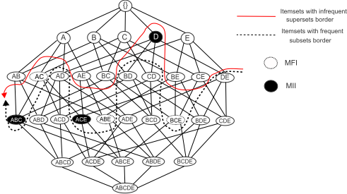
Example 3.1 The lattice in Figure 1 displays the set of itemsets satisfying the constraints FREQUENTSUBS and INFREQUENTSUPERS on the dataset of Table 1 with s = 3. The intersection between both sets is the set MFIs ∪MIIs.
We can then use MODELD,s,b to mine either MFIs or MIIs by simply setting b to true or false. We now define the global constraints FREQUENTSUBS and INFREQUENTSUPERS and we propose propagators.
3.1 The Global Constraint FREQUENTSUBS
We present the new global constraint FREQUENTSUBS used to mine itemsets that have only frequent subsets.
Definition 5 (FREQUENTSUBS) Let x be a vector of Boolean variables, s a support threshold and D a dataset. The global constraint FREQUENTSUBSD,s(x) holds if and only if ∀p ⊂ x-1 (1), freq(p) ≥ s.
Algorithm. The propagator for the global constraint FREQUENTSUBS is presented in Algorithm 1. Algorithm 1 takes as input the variables x and the support threshold s. Algorithm 1 starts by computing the cover of the itemset x-1 (1) and stores it in cover (line 4). Then, for each item j ∈ x-1 (1), Algorithm 1 computes the cover of the subset x-1 (1) \ {j}, and stores it in cov[j] (line 6). If x-1 (1) \ {j} is infrequent then x-1 (1) is not a solution and we return a failure (line 7). Algorithm 1 must then remove items i that cannot belong to a solution containing x-1 (1). To do that, we first test if the itemset x-1 (1) is infrequent (line 8). If so, we remove 1 from dom(xi) for all i ∈ x-1 (∗) (lines 9-10) because the itemset x-1 (1) ∪ {i} has an infrequent subset (x-1 (1)) for every i in x-1 (∗). Otherwise, for every item i in x-1 (∗) we test if the itemset x-1 (1) ∪ {i} is infrequent (line 12). If so, it could have infrequent subsets. Thus, for every item j in x-1 (1), we test if the size of the cover of x-1 (1)∪{i}\{j} (i.e., cov[j]∩cover(i)) is less than s (line 14). If so, we remove i from the possible items, that is, we remove 1 from dom(xi) and break the loop (line 15).
Theorem 2 The propagator in Algorithm 1 enforces domain consistency on the constraint FREQUENTSUBS.
Algorithm 1: Propagator for FREQUENTSUBS
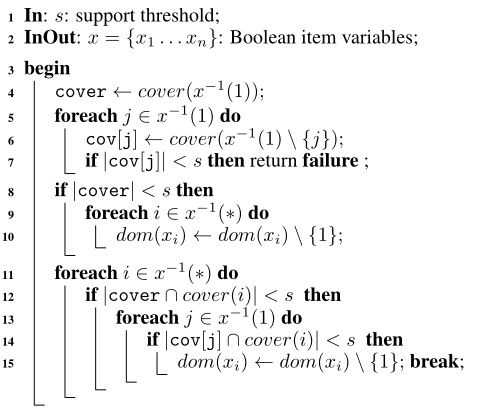
Proof. We first prove that if FREQUENTSUBS admits a solution, x-1 (1) is necessarily one of them. Suppose there is a solution and x-1 (1) is not one of them. This means that there exists a superset of x-1 (1) which has all its subsets frequent. x-1 (1) is one of these subsets. Thus, all subsets of x-1 (1) are frequent and x-1 (1) is solution too, which contradicts the assumption. We now prove that Algorithm 1 returns failure if and only if FREQUENTSUBS does not admit any solution. We know that FREQUENTSUBS has no solution if and only if x-1 (1) is not solution. x-1 (1) is not solution if and only if it has an infrequent subset x-1 (1) \ {j} for some j in x-1 (1). In such a case the test in line 7 is true and failure is returned. If FREQUENTSUBS admits solutions, x-1 (1) is a support for xi = 0, for all i ∈ x-1 (∗). As a result, Algorithm 1 does not need to check consistency of value 0 for any variable.
We now prove that Algorithm 1 prunes value 1 from dom(xi) exactly when i cannot belong to a solution containing x-1 (1). Suppose value 1 of xi is pruned by Algorithm 1. This means that the test in line 8 (or line 14) was true, that is, there exists a subset of x-1 (1) ∪ {i} which is infrequent. Thus, by definition, x-1 (1) ∪ {i} does not belong to any solution. Suppose now that value 1 of xi is not pruned. From lines 8 and 14, we deduce that there does not exist any infrequent subset of x-1 (1)∪{i}. Thus x-1 (1)∪{i} is a solution and value 1 of xi is domain consistent. □
Theorem 3 Given a transaction dataset D of n items and m transactions, Algorithm 1 has an O(n2 ×m) time complexity.
Proof. Computing the size of the cover of an itemset is in O(n×m). Line 5 is called at most n times, leading to a time complexity in O(n2 ×m). The time complexity of lines 8-10 is bounded above by n. The test at line 13 is done at most n2 times. The cover x-1 (1) ∪ {i} \ {j} at line 13 is computed in O(m) thanks to the cov data structure. Thus, the time complexity of lines 9-14 is bounded above by n2 ×m. As a result, Algorithm 1 has an O(n2 ×m) time complexity. □
Algorithm 2: Propagator for INFREQUENTSUPERS
1 In: s: support threshold; 2 InOut: x = {x1 . . . xn}: Boolean item variables; 3 begin 4 cover ← cover(x-1 (1) ∪ x-1 (∗)); 5 if |cover| ≥ s then 6 foreach j ∈ x-1 (0) do 7 if |cover ∩ cover(j)| ≥ s then 8 return failure; 9 foreach i ∈ x-1 (∗) do 10 cover2 ← cover(x-1 (1) ∪ x-1 (∗) \ {i}); 11 if |cover2| ≥ s then 12 foreach j ∈ (x-1 (0) ∪ {i}) do 13 if |cover2 ∩ cover(j)| ≥ s then 14 dom(xi) ← dom(xi) \ {0}; break;3.2 The Global Constraint INFREQUENTSUPERS
We present the new global constraint INFREQUENTSUPERS used to mine itemsets that have only infrequent supersets.
Definition 6 (INFREQUENTSUPERS) Let x be a vector of Boolean variables, s a support threshold and D a dataset. The global constraint INFREQUENTSUPERSD,s(x) holds if and only if ∀p ⊃ x-1 (1), freq(p) < s.
Algorithm. The propagator for the global constraint INFREQUENTSUPERS is presented in Algorithm 2. Algorithm 2 takes as input the variables x and the support threshold s. Algorithm 2 starts by computing cover, the cover of the largest possible itemset, x-1 (1) ∪ x-1 (∗) (line 4). If such an itemset has a frequent superset (line 7) then no itemset containing x-1 (1) can be a solution and we return failure (line 8). Algorithm 2 must then remove value 0 from dom(xi) if the absence of the item i can lead to an itemset that has a frequent superset. To do that, for every free item i (line 9), Algorithm 2 computes cover2, the cover of the largest itemset not containing the item i, i.e. x-1 (1)∪x-1 (∗)\{i} (line 10). If x-1 (1) ∪ x-1 (∗) \ {i} is frequent (line 11), it could have a frequent superset. Thus, for every item j in x-1 (0) ∪ {i} we test whether the itemset x-1 (1) ∪ x-1 (∗) \ {i} ∪ {j} is frequent (line 13). If so, we remove 0 from dom(xi) and break the loop (line 14).
Theorem 4 The propagator in Algorithm 2 enforces domain consistency on the constraint INFREQUENTSUPERS.
Proof. We first prove that if INFREQUENTSUPERS admits a solution, x-1 (1) ∪ x-1 (∗) is necessarily one of them. Suppose there is a solution and x-1 (1) ∪ x-1 (∗) is not one of them. This means that there exists a subset of x-1 (1) ∪ x-1 (∗) which has all its supersets infrequent. x-1 (1) ∪ x-1 (∗) is one of these supersets. Thus, all supersets of x-1 (1) ∪ x-1 (∗) are infrequent and x-1 (1) ∪ x-1 (∗) is solution too, which contradicts the assumption. We now prove that Algorithm 2 returns failure if and only if INFREQUENTSUPERS does not admit any solution. We know that if INFREQUENTSUPERS has solutions, x-1 (1) ∪ x-1 (∗) is one of them. x-1 (1) ∪ x-1 (∗) is not solution if and only if it has a frequent superset. In such a case the test in line 7 is true for some j in x-1 (0) and failure is returned. If INFREQUENTSUPERS has solutions, x-1 (1) ∪ x-1 (∗) is a support for xi = 1, for all i ∈ x-1 (∗). As a result, Algorithm 2 does not need to check consistency of value 1 for any variable.
We now prove that Algorithm 2 prunes 0 from dom(xi) exactly when i belongs to all solutions containing x-1 (1). If the test in line 13 is true this means that with xi = 0 we get itemsets having at least a frequent superset. Hence, 0 must be pruned from dom(xi). Suppose now that the test in line 13 is false for all j. x-1 (1) ∪ x-1 (∗) \ {i} has only infrequent supersets and xi = 0 is domain consistent. □
Theorem 5 Given a transaction dataset D of n items and m transactions, Algorithm 2 has an O(n2 ×m) time complexity.
Proof. Computing the cover of x-1 (1) ∪ x-1 (∗) in line 4 is in O(n × m). The loop in line 6 computes the cover of x-1 (1) ∪ x-1 (∗) ∪ {j} in O(m) using the already computed cover of x-1 (1) ∪ x-1 (∗) (i.e., cover). As a result the worst case time complexity of lines 4-8 is in O(n×m). Similarly, the time complexity of lines 10-14 is bounded above by n ×m. Lines 10-14 are called at most n times, leading to a time complexity in O(n2 × m). □
It is worth noticing the duality between Algorithm 1 and Algorithm 2. Algorithm 1 removes value 1 from dom(xi) if including the item i leads to an itemset having an infrequent subset. Algorithm 2 removes value 0 from dom(xi) if excluding the item i necessarily leads to itemsets having a frequent superset. This duality is not totally obvious at a first glance because Algorithm 1 requires the cov data structure to have its good time complexity whereas Algorithm 2 does not need it. The reason is that Algorithm 1 computes the covers of subsets that we cannot derive from the cover of their supersets whereas Algorithm 2 computes covers of supersets that can be obtained by simple bitwise operation on their subsets.
4 On Constrained Borders
As pointed out in [Bonchi and Lucchese, 2004], constraints can interfere with closedness (or maximality) when they are not monotone. Likewise, constraints can interfere with minimality when they are not anti-monotone. Hence, existing "one-shot" CP approaches can miss solutions because they look for maximal/minimal itemsets that in addition satisfy constraints (see [Lazaar et al., 2016]), whereas we are usually interested in itemsets that are maximal (or minimal) among those satisfying the constraints. In this section we prove that deciding whether a frequent itemset is maximal or closed or minimal among those satisfying the constraints is coNPcomplete. This means that finding maximal/closed/minimal itemsets among those satisfying a set of constraints is coNPhard. It is a proof that it is not possible to solve this problem using a single CSP (unless coNP ⊆ NP). This validates "multi-shot" approaches [Negrevergne et al., 2013].
Theorem 6 Given a dataset D on a set of items I and a set C of user's constraints, deciding whether an itemset is maximal/closed among those satisfying C is coNP-complete.
Proof. Membership. Given an itemset P, a witness to its non maximality/closedness is an itemset P ′ ⊃ P that is frequent, satisfies C, and in the case of closedness has the same frequency as P. Checking that P ′ is frequent and checking that it has the same frequency as P is linear in |D|. Checking that P ′ satisfies C requires the polynomial check of the C constraints. Hence, the "no" answer admits a polynomial certificate, and so deciding maximality or closedness is in coNP.
Completeness. We reduce co3COL, which is coNPcomplete, to the problem of deciding whether an itemset is maximal/closed. We want to decide whether a connected graph G = (V,E) is non colorable with three colors. We build the dataset D on the set I = (a1, . . . , an, b1, . . . , bn, c) of items, where n = |V |. The pair (ai, bi) of items will represent the vertex i in V . D contains the single transaction (1, . . . , 1) and the frequency threshold s is set to |T |/2.
As in all CP models for itemset mining, there is a Boolean variable for each item. The standard semantics is that xp = 1 if and only if the item p is in the itemset returned as solution.
For each edge (i, j) ∈ E, a quaternary constraint c(xai , xbi , xaj , xbj ) is put in the set C of user's constraints. The tuples allowed by c(xai , xbi , xaj , xbj ) are (0000), (0110), (0111), (1001), (1011), (1101), (1110). The assignments (01), (10), and (11) for the pair of variables (xai , xbi ) represent the three colors for vertex i. c(xai , xbi , xaj , xbj ) accepts the tuple (0000) plus the six tuples representing the six combinations of different colors for the pair of vertices (i, j). Hence, by construction, the tuple (0, . . . , 0) is solution, and, as soon as a variable xai or xbi is set to 1, it forces all neighbors in E of vertex i to take another color than the color represented by the assignment of (xai , xbi ). As a result, deciding whether the itemset {c} is maximal/closed among the itemsets satisfying C is equivalent to deciding whether there does not exist any superset of {c} satisfying C, which is equivalent to deciding whether G is non 3-colorable. □
Theorem 7 Given a dataset D on a set of items I and a set C of user's constraints, deciding whether an itemset is minimal/generator among those satisfying C is coNP-complete.
Proof. (Sketch.) Membership is direct adaptation of the proof of membership in Theorem 6: A witness of nonminimality/non-generator of an itemset P is a subset that is infrequent (or has the same frequency in case of generator) and satisfies C, which is polynomial to check. Completeness is the dual of the reduction in Theorem 6. We reduce co3COL to the problem of deciding whether an itemset is minimal/generator. We build the dataset D on the set I = (a1, . . . , an, b1, . . . , bn) of items with the three transactions (1, 0, . . . , 0), (0, . . . , 0, 1) and (1, . . . , 1). The frequency threshold s is set to |T |/2. For each edge in the graph, we use again a quaternary constraint but the tuple (0000) is replaced by the tuple (1111) and the three colors are represented by the assignments (00), (01), and (10) instead of (01), (10), and (11). By construction, the tuple (1, . . . , 1) is solution and deciding whether the itemset (a1, . . . , an, b1, . . . , bn) is minimal/generator among the itemsets satisfying C is equivalent to deciding whether there does not exist any subset of (a1, . . . , an, b1, . . . , bn) satisfying C, which is equivalent to deciding whether G is non 3-colorable. □
Corollary 1 Given a dataset D on a set of items I and a set C of user's constraints, finding an itemset that is maximal/closed/minimal/generator among those satisfying C is coNP-hard.
5 Experiments
We made several experiments to compare our CP model MODELD,s,b to the state of the art approaches.
5.1 Experimental Protocol
The implementation of MODELD,s,b and its constraint propagators were carried out in the Oscar solver using Scala (bitbucket.org/oscarlib/oscar). The code is publicly available at gite.lirmm.fr/belaid/cp4borders. All experiments were conducted on an Intel core i7, 2.2Ghz with a RAM of 8Gb and a timeout of one hour. MODELD,s,b is denoted by CP4MFI (resp. CP4MII) when b = 1, i.e. mining MFIs, (resp. b = 0, mining MIIs). We used the global constraint COVERSIZE to encode the constraint (3) in MODELD,s,b. COVERSIZED(x, p) holds if and only if p = |cover(x-1 (1))| [Schaus et al., 2017]. We enforce frequency by simply adding the constraint p ≥ s and infrequency by adding p < s. The propagator of COVERSIZE enforces DC on the frequency, but it does not on the infrequency. We have assessed the quality of the COVERSIZE encoding of infrequency by comparing to a propagator that enforces DC on the infrequency. We observed that the number of additional nodes explored with the COVERSIZE encoding was marginal and the CPU time was better. We thus use the propagator of COVERSIZE in all our experiments. As an MFI is a closed itemset and an MII is a generator, we enhance propagation by adding, respectively, the global constraints COVERCLOSURE [Schaus et al., 2017] and GENERATOR [Belaid et al., 2019]. After a few preliminary tests, we decided to use smallest item frequency first as variable ordering heuristic and largest value first as value ordering heuristic. We compared CP4MFI to the FPGROWTH [Grahne and Zhu, 2003] specialized algorithm for extracting MFIs (Borgelt's platform: borgelt.net/fpgrowth.html) and CP4MII to WALKY-G [Szathmary et al., 2012] for mining MIIs (CORON platform: coron.loria.fr). We selected several real-sized datasets from the FIMI repository (fimi.ua.ac.be/data). A dataset is characterized by its name, the number of items |I|, the number of transactions |T | and its density ρ.
5.2 Mining Borders
Our first experiment compares CP4MFI to FPGROWTH and CP4MII to WALKY-G for mining MFIs and MIIs. For each approach and each selected instance, Table 2 reports the CPU time and the number of MFIs/MIIs. 1 An instance of a given dataset is characterized by its minimum support s (e.g., Zoo 50 denotes the instance of Zoo with s = 50).
A first observation is that the specialized algorithms FPGROWTH and WALKY-G follow a completely different approach to extract MFIs and MIIs whereas our CP model can T10 = T10I4D100K TO= timeout OOM= out of memory mine a border or the other just by flipping a parameter. When mining MFIs, the main observation that we can draw from Table 2 is that, as expected, the specialized algorithm FPGROWTH performs very well. However, CP4MFI is very competitive too, and even faster on one instance (Chess 160). As for MIIs, CP4MII outperforms WALKY-G in 14 instances out of 26. CP4MII reaches once the timeout of one hour. WALKYG reaches the time out on two instances and an out of memory state on three instances. WALKY-G uses a hash structure for storing frequent generators. Maintaining this data structure can be very expensive, especially on dense datasets. For instance, on the very dense Chess 500, WALKY-G exhausts the 8Gb of memory to store the 50M frequent generators. On the moderately dense Connect 7000, WALKY-G needs to store more than 7.4M frequent generators to find the 165K MIIs in 163.25 seconds. On these two instances, CP4MII returns the whole set of MIIs in only 97.42 and 99.42 seconds, respectively. On sparse datasets, where we have few frequent generators, WALKY-G is very efficient. On the very sparse dataset T10, WALKY-G stores less than 50K frequent generators to extract the 698K MIIs of T10 50 in less than 5 seconds whereas CP4MII needs more than 7 minutes.
1 This number is computed by releasing the timeout.
| Dataset |I| × |T | | s | Mining MFIs | Mining MIIs | ||||
|---|---|---|---|---|---|---|---|
| ρ(%) | FPGROWTH | CP4MFI | #MFIS | WALKY-G | CP4MII | #MIIS | |
| Zoo 36 × 101 44% | 50 | 0.01 | 0.03 | 32 | 0.12 | 0.04 | 111 |
| 9 | 0.01 | 0.08 | 200 | 0.10 | 0.13 | 875 | |
| 1 | 0.01 | 0.09 | 59 | 0.27 | 0.12 | 1,071 | |
| Vote 48 × 435 33% | 150 | 0.01 | 0.04 | 75 | 0.19 | 0.10 | 479 |
| 5 | 0.08 | 0.77 | 13,787 | 0.85 | 1.40 | 37,526 | |
| 1 | 0.13 | 0.47 | 342 | 1.26 | 1.24 | 32,067 | |
| Anneal 93 × 812 45% | 700 | 0.01 | 0.05 | 65 | 0.26 | 0.08 | 303 |
| 100 | 0.42 | 1.10 | 15,889 | 9.59 | 2.06 | 77,119 | |
| 50 | 0.61 | 1.13 | 14,296 | 23.48 | 3.41 | 86,783 | |
| Chess 75 × 3, 196 49% | 2,500 | 0.01 | 0.10 | 286 | 0.10 | 0.13 | 511 |
| 1,000 | 1.04 | 4.34 | 114,382 | 23.14 | 8.38 | 152,316 | |
| 500 | 16.60 | 25.66 | 952,812 | OOM | 97.42 | 1,353,344 | |
| 160 | 233.78 | 127.30 | 5,784,232 | OOM | 923.84 | 9,364,262 | |
| Mushroom 119 × 8, 124 19% | 4,000 | 0.01 | 0.03 | 12 | 0.31 | 0.06 | 145 |
| 40 | 0.07 | 1.09 | 12,010 | 0.86 | 2.33 | 48,111 | |
| 4 | 0.24 | 1.56 | 39,416 | 1.95 | 4.58 | 49,046 | |
| Connect 129 × 67, 557 33% | 55,000 | 0.01 | 0.51 | 594 | 0.34 | 0.48 | 891 |
| 7,000 | 2.60 | 69.03 | 123,345 | 163.25 | 99.42 | 165,198 | |
| 2,000 | 24.40 | 342.95 | 893,826 | TO | 885.99 | 1,180,278 | |
| 676 | 102.90 | 800.65 | 3,283,735 | TO | 3541.77 | 4,221,496 | |
| T10 1, 000 × 100, 000 1% | 5,000 | 0.01 | 0.19 | 10 | 0.13 | 4.59 | 905 |
| 1,000 | 0.12 | 207.89 | 307 | 2.33 | 373.01 | 344,651 | |
| 50 | 0.35 | 255.18 | 12,062 | 4.27 | 472.82 | 698,556 | |
| Pumsb 2, 113 × 49, 046 3% | 48,000 | 0.01 | 0.09 | 3 | 0.25 | 10.18 | 2,115 |
| 32,000 | 0.21 | 470.80 | 17,791 | 30.10 | 48.55 | 57,425 | |
| 17,000 | 145.96 | TO | 2,403,260 | OOM | TO | > 3×10⁶ | |
Table 2: FPGROWTH vs CP4MFI for mining MFI and WALKY-G vs CP4MII for mining MIIs (time in seconds)
5.3 Mining Constrained Borders
In many practical applications, the user asks for itemsets satisfying some additional constraints. We performed experiments that show the strength of our CP approach in taking into account user's constraints. We look for MFIs of minimim size lb and MIIs of maximum size ub. These two queries can easily be expressed in our CP model by adding the cardinality constraints ∑i∈I xi ≥ lb to CP4MFI, and ∑i∈I xi ≤ ub to CP4MII. FPGROWTH includes a filtering step allowing us to specify the minimum size of extracted MFIs. However, WALKY-G does not provide such feature, and extracting MIIs under cardinality constraints is only possible via a post-processing step. Table 3 reports the results. We selected the instances having more than one million MFIs and/or MIIs in Table 2. For each selected instance, we increased lb (resp.
| Instance | Mining constrained MFIs | Mining constrained MIIs | ||||||
|---|---|---|---|---|---|---|---|---|
| lb | FPGROWTH | CP4MFI | #SOL | ub | WALKY-G | CP4MII | #SOL | |
| Chess 500 | 25 24 21 17 | 17.97 17.60 16.60 17.86 | 0.30 0.72 1.65 10.58 | 0 2 2,091 171,567 | 1 3 5 7 | OOM OOM OOM OOM | 0.08 0.41 8.88 16.58 | 19 1,962 31,591 224,172 |
| Chess 160 | 29 28 26 23 | 201.55 224.31 226.77 219.82 | 1.23 1.73 3.51 16.08 | 0 10 1,527 132,814 | 1 3 4 6 | OOM OOM OOM OOM | 0.03 0.62 1.31 17.44 | 9 2,384 13,487 186,653 |
| Connect 676 | 40 33 32 31 | 117.87 111.95 109.07 125.62 | 5.96 69.00 117.17 171.04 | 0 266 21,788 157,793 | 1 2 4 5 | TO TO TO TO | 0.15 2.53 22.81 119.42 | 20 1,612 33,742 144,007 |
| Pumsb 17000 | 35 30 26 22 | 157.28 157.58 153.33 154.52 | 1.16 14.96 148.26 3019.25 | 0 21 1,663 55,018 | 1 3 6 8 | OOM OOM OOM OOM | 4.59 11.94 254.58 2702.20 | 2,033 5,721 166,178 1,388,040 |
TO= timeout OOM= out of memory
Table 3: FPGROWTH vs CP4MFI for mining constrained MFI and WALKY-G vs CP4MII for mining constrained MIIs (time in seconds)
decreased ub) and we report the CPU time, in seconds, according to the number of solutions.
The main observation on the performance of FPGROWTH for extracting constrained MFIs is that its CPU time is almost constant. For instance, extracting more than 5M or just 10 MFIs on Chess 160 requires almost the same CPU time. This is explained by the fact that the cardinality constraint in FPGROWTH has no pruning power. It is just used as a checker. On the contrary, when lb increases, CP4MFI removes more values thanks to constraint propagation, thus drastically reducing the search space. Take for instance Pumsb 17000. When lb = 22, CP4MFI extracts the 55K MFIs in more than 50 minutes whereas when lb increases to 30, CP4MFI returns the 21 remaining solutions in only 15 seconds. On instances with no solutions, such as Pumsb 17000 with lb = 35, CP4MFI proves the absence of solutions in one second whereas FPGROWTH spends 157.28 seconds.
For WALKY-G, no results are reported because it already has an OOM or TO state before reaching post-processing step. The main observation that we can draw on the behavior of CP4MII is again the strong correlation between the increase of tightness of the cardinality constraint (that is, the decrease of ub) and the drop in CPU time needed to extract the constrained MIIs. The explanation for this good behavior of CP4MII is again the strength of constraint propagation to discard inconsistent values, thus reducing the search space. On Pumsb 17000, when ub decreases from 8 down to 1, CP4MII goes from 45 minutes down to 4.59 seconds to return the set of MIIs (1.3M MIIs for ub = 8 and 2K MIIs for ub = 1).
6 Conclusion
We have presented a CP model for mining MFIs and MIIs. We defined two new global constraints, namely FREQUENTSUBS and INFREQUENTSUPERS, with polynomial complete propagators. We have proved that the problem of MFIs or MIIs with constraints is co-NPhard, ruling out the hope for a single CSP solving this problem. Nevertheless, our CP model is sound when the additional constraints are monotone on MFIs or anti-monotone on MIIs. Experiments showed that the CP approach is competitive with state of the art techniques for mining MFIs or MIIs and even better for mining MFIs or MIIs with additional constraints.
@inproceedings{ijcai2019p149,
  title     = {Constraint Programming for Mining Borders of Frequent Itemsets},
  author    = {Belaid, Mohamed-Bachir and Bessiere, Christian and Lazaar, Nadjib},
  booktitle = {Proceedings of the Twenty-Eighth International Joint Conference on
               Artificial Intelligence, {IJCAI-19}},
  publisher = {International Joint Conferences on Artificial Intelligence Organization},
  editor    = {Sarit Kraus},
  pages     = {1064--1070},
  year      = {2019},
  month     = {8},
  note      = {Main track},
  doi       = {10.24963/ijcai.2019/149},
  url       = {https://doi.org/10.24963/ijcai.2019/149},
}
TY - CPAPER TI - Constraint Programming for Mining Borders of Frequent Itemsets AU - Belaid, Mohamed-Bachir AU - Bessiere, Christian AU - Lazaar, Nadjib T2 - Proceedings of the Twenty-Eighth International Joint Conference on Artificial Intelligence, IJCAI-19 PB - International Joint Conferences on Artificial Intelligence Organization PY - 2019 SP - 1064 EP - 1070 DO - 10.24963/ijcai.2019/149 UR - https://doi.org/10.24963/ijcai.2019/149 ER -Copied
Machine-readable versions of this paper, for tools and AI agents:





