
Binarized Neural Networks for Resource-Efficient Hashing with Minimizing Quantization Loss
Proceedings of the Twenty-Eighth International Joint Conference on Artificial Intelligence. Main track. Pages 1032-1040.
https://doi.org/10.24963/ijcai.2019/145
Keywords
- Computer Vision: Recognition: Detection, Categorization, Indexing, Matching, Retrieval, Semantic Interpretation
- Computer Vision: Computer Vision
Abstract
In order to solve the problem of memory consumption and computational requirements, this paper proposes a novel learning binary neural network framework to achieve a resource-efficient deep hashing. In contrast to floating-point (32-bit) full-precision networks, the proposed method achieves a 32x model compression rate. At the same time, computational burden in convolution is greatly reduced due to efficient Boolean operations. To this end, in our framework, a new quantization loss defined between the binary weights and the learned real values is minimized to reduce the model distortion, while, by minimizing a binary entropy function, the discrete optimization is successfully avoided and the stochastic gradient descend method can be used smoothly. More importantly, we provide two theories to demonstrate the necessity and effectiveness of minimizing the quantization losses for both weights and activations. Numerous experiments show that the proposed method can achieve fast code generation without sacrificing accuracy.
- [Courbariaux and Bengio, 2015] Matthieu Courbariaux and Yoshua Bengio. Binaryconnect: Training deep neural net- works with binary weights during propagations. In NIPS, pages 3123-3131, 2015.
- [Courbariaux et al., 2016] Matthieu Courbariaux, Itay Hubara, Daniel Soudry, Ran El-Yaniv, and Yoshua Ben- gio. Binarized neural networks: Training neural networks with weights and activations constrained to +1 or 1. In NIPS, pages 4114-4122, 2016.
- [Do et al., 2016] Thanh-Toan Do, Anh-Dzung Doan, and Ngai-Man Cheung. Learning to hash with binary deep neural network. In ECCV, pages 219-234, 2016.
- [Farenzena et al., 2010] Michela Farenzena, Loris Bazzani, Alessandro Perina, Vittorio Murino, and Marco Cristani. Person re-identification by symmetry-driven accumulation of local features. In CVPR, pages 2360-2367, 2010.
- [Gong et al., 2013] Yunchao Gong, Svetlana Lazebnik, Al- bert Gordo, and Florent Perronnin. Iterative quantization: A procrustean approach to learning binary codes for large- scale image retrieval. IEEE TPAMI, 35(12):2916 -2929, 2013.
- [Han et al., 2015] Song Han, Jeff Pool, John Tran, and William J. Dally. Learning both weights and connections for efficient neural network. In NIPS, pages 1135-1143, 2015.
- [Heo et al., 2015] Jae-Pil Heo, Youngwoon Lee, Junfeng He, Shih-Fu Chang, and Sung-Eui Yoon. Spherical hashing: Binary code embedding with hyperspheres. IEEE TPAMI, 37(11):2304-2316, 2015.
- [Hinton et al., 2015] Geoffrey Hinton, Oriol Vinyals, and Jeff Dean. Distilling the knowledge in a neural network. In arXiv preprint arXiv:1503.02531, 2015.
- [Hou et al., 2017] Lu Hou, Quanming Yao, and James T. Kwok. Loss-aware binarization of deep networks. In ICLR, 2017.
- [Huang et al., 2016] Chen Huang, Chen Change Loy, and Xiaoou Tang. Unsupervised learning of discriminative at- tributes and visual representations. In CVPR, pages 5175- 5184, 2016.
- [Indyk and Motwani, 1998] Piotr Indyk and Rajeev Mot- wani. Approximate nearest neighbors: towards remov- ing the curse of dimensionality. In STOC, pages 604-613, 1998.
- [Krizhevsky and Hinton, 2009] Alex Krizhevsky and Geof- frey Hinton. Learning multiple layers of features from tiny images. Technical report, University of Toronto, 2009.
- [Krizhevsky et al., 2012] Alex Krizhevsky, Ilya Sutskever, and Geoffrey E. Hinton. Imagenet classification with deep convolutional neural networks. In NIPS, pages 1097- 1105, 2012.
- [Lai et al., 2015] Hanjiang Lai, Yan Pan, Ye Liux, and Shuicheng Yan. Simultaneous feature learning and hash coding with deep neural networks. In CVPR, pages 3270- 3278, 2015.
- [Li et al., 2016] Fengfu Li, Bo Zhang, and Bin Liu. Ternary weight networks. In Workshop in NIPS, 2016.
- [Liny et al., 2016] Kevin Liny, Jiwen Luz, Chu-Song Cheny, and Jie Zhou. Learning compact binary descriptors with unsupervised deep neural networks. In CVPR, pages 1183-1192, 2016.
- [Liong et al., 2015] Venice Erin Liong, Jiwen Lu, Gang Wang, Pierre Moulin, and Jie Zhou. Deep hashing for compact binary codes learning. In CVPR, pages 2475- 2483, 2015.
- [Liu et al., 2016a] Haomiao Liu, Ruiping Wang, Shiguang Shan, and Xilin Chen. Deep supervised hashing for fast image retrieval. In CVPR, pages 2064-2072, 2016.
- [Liu et al., 2016b] Xinchen Liu, Wu Liu, Tao Mei, and Huadong Ma. A deep learning-based approach to pro- gressive vehicle re-identification for urban surveillance. In ECCV, pages 869-884, 2016.
- [Perpinan and Raziperchikolaei, 2015] Miguel A. Carreira Perpinan and Ramin Raziperchikolaei. Hashing with bi- nary autoencoders. In CVPR, pages 557-566, 2015.
- [Rastegariy et al., 2016] Mohammad Rastegariy, Vicente Ordonezy, Joseph Redmon, and Ali Farhadi. Xnor-net: Imagenet classification using binary convolutional neural networks. In ECCV, pages 525-542, 2016.
- [Schrof et al., 2015] Florian Schrof, Dmitry Kalenichenko, and James Philbin. Facenet: A unified embedding for face recognition and clustering. In CVPR, pages 815-823, 2015.
- [Shen et al., 2015] Fumin Shen, Chunhua Shen, Wei Liu, and Heng Tao Shen. Supervised discrete hashing. In CVPR, pages 37-45, 2015.
- [Simonyan and Zisserman, 2015] Karen Simonyan and An- drew Zisserman. Very deep convolutional networks for large-scale image recognition. In ICLR, 2015.
- [Szegedy et al., 2015] Christian Szegedy, Wei Liu, Yangqing Jia, Pierre Sermanet, Scott Reed, Dragomir Anguelov, Du- mitru Erhan Vincent Vanhoucke, and Andrew Rabinovich. Going deeper with convolutions. In CVPR, pages 1-9, 2015.
- [van de Weijer et al., 2007] Joost van de Weijer, Cordelia Schmid, Jakob Verbeek, and Diane Larlus. Learning color names for real-world applications. In CVPR, 2007.
- [Venkateswara et al., 2017] Hemanth Venkateswara, Jose Eusebio, Shayok Chakraborty, and Sethuraman Pan- chanathan. Deep hashing network for unsupervised do- main adaptation. In CVPR, pages 5018-5027, 2017.
- [Wang et al., 2012] Jun Wang, Sanjiv Kumar, and Shih-Fu Chang. Semi-supervised hashing for large-scale search. IEEE TPAMI, 34(12):2393-2406, 2012.
- [Weiss et al., 2009] Yair Weiss, Torralba, and Rob Fergus. Spectral hashing. In NIPS, pages 1753-1760, 2009.
- [Yan et al., 2007] Shuicheng Yan, Dong Xu, Benyu Zhang, Hong jiang Zhang, Qiang Yang, and Stephen Lin. Graph embedding and extensions: A general framework for di- mensionality reduction. IEEE TPAMI, 29(1), 2007.
- [Zhao et al., 2013a] Rui Zhao, Wanli Ouyang, and Xiaogang Wang. Person re-identification by salience matching. In ICCV, pages 2528-2535, 2013.
- [Zhao et al., 2013b] Rui Zhao, Wanli Ouyang, and Xiaogang Wang. Unsupervised salience learning for person re- identification. In CVPR, pages 3586-3593, 2013.
- [Zhao et al., 2014] Rui Zhao, Wanli Ouyang, and Xiao- gang Wang. Learning mid-level filters for person re- identification. In Proc. CVPR, pages 144-151, 2014.
- [Zhao et al., 2015] Fang Zhao, Yongzhen Huang, Liang Wang, and Tieniu Tan. Deep semantic ranking based hash- ing for multi-label image retrieval. In CVPR, pages 1556- 1564, 2015.
- [Zheng et al., 2015] Liang Zheng, Liyue Shen, Lu Tian, Shengjin Wang, Jingdong Wang, and Qi Tian. Scalable person re-identification: A benchmark. In ICCV, pages 1116-1124, 2015.
- [Zhou et al., 2016] Shuchang Zhou, Yuxin Wu, Zekun Ni, Xinyu Zhou, He Wen, and Yuheng Zou. Dorefa-net: Train- ing low bitwidth convolutional neural networks with low bitwidth gradients. In arXiv:1606.06160, 2016.
- [Zhu et al., 2016] Han Zhu, Mingsheng Long, Jianmin- Wang, and Yue Cao. Deep hashing network for efficient similarity retrieval. In AAAI, pages 2415-2421, 2016.
- [Zhu et al., 2017] Chenzhuo Zhu, Song Han, Huizi Mao, and William J. Dally. Trained ternary quantization. In LCLR, 2017.
References were extracted automatically from the PDF and may contain errors.
Full text extracted automatically from the PDF; figures, tables and equations may differ. The PDF is the version of record.
1 Introduction
Binary embedding (hashing) is widely used to address a variety of large-scale computer vision and machine learning problems due to its advanced performance in both data compression and fast approximate nearest-neighbour search. The basic requirement of binary embedding (hashing) is that the measurements in code space should be consistent with the measurements in original space and that consistency makes it feasible for similar samples to have similar binary codes. In order to achieve this, various learning hash methods have been proposed to explore data-dependent hash functions. Among them, deep hashing [Venkateswara et al., 2017; Huang et al., 2016; Liny et al., 2016; Lai et al., 2015; Perpinan and Raziperchikolaei, 2015; Zhao et al., 2015; Liong et al., 2015] would be the most anticipated method, because of the advanced non-linearity and memorability to capture consistency.
∗To whom all correspondence should be addressed.
However, despite the satisfied results achieved by recent deep hashing-based methods, deep neural networks (DNN) often encounter unbearable memory consumption and computational requirements during the inference phase. This makes it difficult to deploy DNN-based applications on low cost devices. Taking VGG-16 [Simonyan and Zisserman, 2015] as an example, it consists of 138 million parameters and the computational complexity of the reasoning stage is very large. However, the biggest advantage of hashing is to reduce storage space and improve efficiency. In a sense, using a DNN for hashing is a dilemma. Thus, it is necessary to speed up code generation and reduce storage consumption.
Recently, some compression strategies, such as pruning [Han et al., 2015], binarization [Courbariaux and Bengio, 2015] and distillation [Hinton et al., 2015], have been explored to reduce the floating-point multiplication in convolutions. Among them, binarization of neural network will be the most economical method, because each weight only needs one bit. It can significantly reduce storage and eliminate multiplication, but unfortunately some problems are inevitably introduced into neural networks. The immediate suffering is to incorporate the sign function into the neural network. Since the step function is not differentiable, it is difficult to propagate the gradient backwards to update the parameters. The more important problem is that most existing compression methods cannot consider the quantization loss between the binary model used for inference and the actual trained real-valued model.
Driven by these two perspectives, we develop a novel framework, which can minimize the quantization loss for the weights and activations (see Fig. 1), to learn a binary neural network for Resource-Efficient Deep Hashing (REDH). Compared with existing deep hashing methods, the proposed binary network can speed up code generation and reduce storage consumption. This is because Boolean operations are used in our architecture. First, we use the log cosh function to define the quantization loss between the real-valued weight and its quantized code. By minimizing this loss, the realvalued weights learned can approximate the amount of code that is quantized. Therefore, this allows us to directly train the deep architecture of real values using the classical stochastic gradient descent (SGD) and successfully avoids the problem of the sign function. Since the difference between binary and real weights has been minimized, the binary architecture used can still retain the original attributes. Our theoretical analysis shows that the vibration of the output representation can be bounded by the proposed quantization loss. Second, we use the binary entropy function to further define the quantitative loss between activation and its quantified code. By minimizing the difference (loss) between them, we can get the binary input in the middle layer, so the multiplication in the convolution can be replaced by the XNOR operand. At the same time, the activation of the middle layer and the final binary representation can be treated equally, so the gradient can propagate backwards in the same way. We provide a theory to show that an auxiliary distance converges to the Hamming distance uniformly under the control of quantization loss. Moreover, various properties or constraints used in other classical hashing methods can be seamlessly integrated into our framework. Finally, by optimizing the integrated objective function, a binary neural network can be constructed to fast generate binary codes for some special tasks.
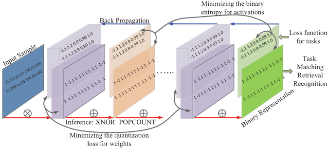
In summary, we make the following contributions: 1) To the best of our knowledge, we are the first to integrate the learning of a binary neural network and the generation of binary codes into a unified framework. 2) In order to learn the network directly on the real values, we propose the quantization losses for the weights and activations. 3) We provide two theories: Theoretically prove the necessity of minimizing the weight quantization loss and positively ensure that the Hamming distance can be safely replaced by an auxiliary distance. 4) A large number of experiments show that the proposed method can improve the efficiency of code generation, but without sacrificing much accuracy.
2 RelatedWork
Recently, due to the promising results in the area of object recognition, DNNs [Venkateswara et al., 2017; Huang et al., 2016; Liny et al., 2016; Lai et al., 2015; Perpinan and Raziperchikolaei, 2015; Zhao et al., 2015; Liong et al., 2015] have been also introduced to learn binary codes. In [Liong et al., 2015], multiple hierarchical non-linear transformations are used to learn binary codes. In the same year, [Zhao et al., 2015] also incorporates deep convolutional neural network into hash functions. In addition, a binary auto-encoder model which seeks to reconstruct an image from the binary code is proposed in [Perpinan and Raziperchikolaei, 2015]. While [Lai et al., 2015] focuses on using a deep architecture for supervised hashing, in which three blocks including a stack of convolution layers, a divide-and-encode module and a triplet ranking loss are designed. In [Liny et al., 2016], an unsupervised deep neural network is proposed to learn binary descriptors. [Huang et al., 2016] trains deep convolutional neural networks coupled with unsupervised discriminative clustering and then uses the cluster membership as a soft supervision. Actually, the deep hashing network can also exploited for unsupervised domain adaptation [Venkateswara et al., 2017]. Undoubtedly, these methods achieve better results than the linear methods. However, a significant disadvantage of deep neural networks is that inference (code generation) is computationally expensive and memory intensive. In this paper, our goal is to propose a binary neural network to solve this problem.
Using binary neural networks to reduce unbearable burden of computation and memory is an active research topic. [Courbariaux and Bengio, 2015] proposes a simple method to binarize the network weights. Later, they extend this work to binarize the activations as well [Courbariaux et al., 2016]. XNOR-Networks [Rastegariy et al., 2016], in which both weights and activations are binarized, results in 58 times faster convolutional operations and 32 times memory savings. Following the XNOR-Networks, [Hou et al., 2017] further consider the effect of binarization on a loss during binarization. It is worth noting that the loss in [Hou et al., 2017] is not the quantization loss discussed in our paper. DoReFa-Net [Zhou et al., 2016] also binarizes weights into bits but quantizes both gradients and activations into low bitwidth codes. Another similar line is to train ternary weight networks [Li et al., 2016; Zhu et al., 2017] which weights are constrained to +1, 0 and -1. The ternary weight networks (TWNs) [Li et al., 2016] are designed to reduces the accuracy loss of binary networks by introducing zero as a third quantized value. Based on TWNs, Zhu et. al. [Zhu et al., 2017] quantize the weights into 0 and two real-values (positive and negative) for each layer, which are trainable parameters. However, these methods all focus on training compressed networks for the task of recognition. As far as we know, there is no algorithm for efficient hashing. Moreover, the quantization loss between the quantized codes and the full precision weights has not been considered in training, which is potentially harmful for the performance after the network quantization.
3 The Proposed Binarized Hashing Network
In this paper, we consider to directly learn deep binary neural networks for binary representation and simultaneously minimize the quantization loss between the real-valued parameter learned and the final binary code that is quantized. Generally, state-of-the-art deep architectures consist of billions of operands in convolutions and activations which are computationally expensive and memory consumption in inference. In this section, we first discuss the scheme of binarizing the convolution weights and then propose a method of binarizing the output of the activation. Finally, we introduce the basic requirements of binary embedding.
Let F be a DNN with L layers, I be a raw sample input of the network, Wl be a matrix (or tensor) of the real-valued parameters in the lth layer and xl be the output of the lth layer. Thus, we have xL = F(I) which is the final binary representation of the sample I and x0 = I which is the input of the network. Simply, for all the layers including the input and the output, we can write the operations as:
where B is a binary function and A is a activation function both which will are discussed later. It is worth noting that ⊕ denotes the xnor + popcount operation. In fact, in the inference, the binarization can be conducted in advance and only the binary nets need to be stored in memory.
3.1 BinarizingWeights
In fact, convolution is the most basic operation in deep networks, and the size of the parameters leads to a lot of time and memory consumption. Therefore, our first step is to binarize the real-value weights into bits and replace multiplications with xnor + popcount operations.
Binarization
Configuring the parameters using binary codes {-1, 1} directly would be the most straightforward method but it is obvious that discrete optimization for the parameter configuration is an NP-hard problem. Otherwise, the most feasible solution is that the real-valued parameters is first learned and then weights binarization is performed by transforming real values to 1 and -1 as:
where B(·) is an element-wise function. Other compression methods could project their parameters into clusters and thus the parameters in the same cluster share their representative quantized values. For example, ternary values [Zhu et al., 2017] are adopted to represent the parameters by introducing a threshold and [Zhou et al., 2016] uses a straight-through estimator method to generate low bitwidth weights. In contrast, sign function in Eq. 1 can produce the most efficient operations and the most compact representations.
Minimizing Quantization Loss
However, most existing methods try to generate a low bitwidth weight as close as possible to the original method, but the quantization loss between the final binary network and the real valued parameters cannot be minimized during the training. Thus, it is inevitable to explore a variety of complex quantization schemes that will increase the complexity of the model. Instead, we think a better network of realvalued weights that is closer to the final quantized value can be first learned and then the following quantification becomes a simple matter.
Before introducing the quantization loss, we give a simple example to illustrate the importance of minimizing the loss. Given a network of L layers without regard to activations, we have the following theory:
Theorem 3.1. Suppose x∗l (k) = 〈W k l , xl-1〉 and xl(k) = 〈sign(W k l ), xl-1〉 for the kth neuron in the lth layer, then we can define ∆xl(k) = xl(k) - x∗l (k) ∆W k l = W k l - sign(W k l ). If we define Θ = supi,k ||xl||2 , the following inequality holds
All the proofs will be provided in an anonymous website (https://github.com/AI-2019/IJCAI2019.git).
We can see that the vibrations (loss) of weights ||∆Wl|| are transmitted on the networks to the output xL. Furthermore, the inequality in Theory 3.1 clearly demonstrates that minimizing ||∆Wl||, l = 1, · · · ,L can reduce the vibration of output ||∆xL||. Although we provide the theory for the simplified networks, the same conclusion can be also obtained for the complex models which activation functions are used. This is because that, normally, the activation functions are monotonically non-decreasing. While the robustness of final representation xL is very significant for the following tasks. Thus, to improve the robustness, we need to minimize the quantization loss of weights.
To this end, we explore a novel quantization loss to guide the training of parameters. Considering the absolute function |x| ≈ log(cosh(x)), we can define our quantization loss as:
where U has the same size of Wl and all items in U are 1 and ⊗ is the convolution operation playing the same role as summation here. Both log(·) and cosh(·) are element-wise functions. It is obvious that the loss function L(Wl) is differentiable and has two minimums for each item of Wl. The following theory guarantees that ||∆Wl||2 in Theory 3 can be bounded by the proposed quantization loss.
Theorem 3.2. If we define ∆Wl = Wl - sign(Wl) and a loss function in Eq. 4, the following inequality holds:
It is obvious that U is a constant matrix. As a result, minimizing L(Wl) can make parameters move to the representative quantized values {-1, 1} with a large probability and further reduce the output vibrations ||∆xL||2 .
3.2 Binarizing Activations
Binarizing weights into bits converts the convolutional multiplication to a real-value addition that is still slower than the xnor operation. To further accelerate the inference, we also need to binarize the activation of middle layers. In fact, we can think of the output of activations as being the same as the final binary representation.
Binarization
Assume that B(W k l ) and the binary representation in the last layer xl-1 are given. To simulate the real-valued convolutions for kth neuron, we use ⊕ operator which is defined as:
where Y k l = B(W k l ) xnor xl-1 is a vector with the same size of W k l . In fact, all filters W k l have the same size to xl-1. Thus, zl(k) ∈ [-dwl , dwl ] is a value centred at 0 and has the largest norm that is the same to the size dwl of W k l .
In this paper, we adopt a logistic function pl(k) = σ(zl(k)) = 1 1+exp(-ηzl(k)) as the activation function in our binary neural networks, in which the steepness of the curve η is set to 1. Thus, the activations pl(k) can be considered as a probability of the kth neuron at the lth layer. Moreover, it is easy to prove that the expectation of activations is u = 0.5. Therefore, by using the sign step function again, our stochastic binarization function is defined as:
The quantization procedure will be conducted for the output representation layer and all the intermediate layers xl : l = 1, · · · ,L. In summary, the activation function of our realvalued net in the training stage is A(·) = 2σ(·) - 2u whilst the intermediate layers of the corresponding binary net in the inference stage is xl(k) = sign(A(zl(k))).
Minimizing Binary Entropy
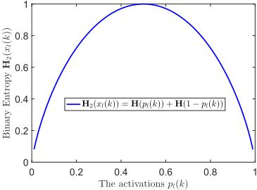
Obviously, the quantization step speeds up the convolutions but suffers from the information loss which would make the learned model unstable. For example, when pl(k) is very close to u, the binarization decision is very sensitive. To mitigate the negative influence, we consider the quantization procedure as a Bernoulli process of the random variable xl(k). Thus, simply, we have Pr(xl(k) = 1) = pl(k) and Pr(xl(k) = -1) = 1 - pl(k). Therefore, a binary entropy function H2(xl(k)) (See Fig. 2) of xl(k) can be given by:
where H(pl(k)) = -pl(k) log2(pl(k)) is the entropy of the probability pl(k). We can observe that the maximum of binary entropy function H2 attains its maximum value, when pl(k) = 0.5. On the contrary, minimizing the binary entropy function will make pl(k) closer to either 1 or 0. Therefore, based on the Bernoulli process of activations, we can define the quantization loss for binarizing the activations as:
Directly real-valued network training that minimizes quantization loss avoids the difficulties caused by discrete variables. More importantly, we will theoretically prove that minimizing the quantization loss of last layer can ensure that an auxiliary distance in the learning space consistently approaches the expected Hamming distance. Therefore, it is feasible to use a differentiable distance to replace the Hamming distance in objectives for hash learning. Finally, the stochastic gradient descent method can be used smoothly.
Balance and Independence
Beside our proposed quantization losses, similar to most other hashing methods [Weiss et al., 2009; Liong et al., 2015], we also add a regularization item to consider the bit balance and independence of the activation for each layer as:
where Pl consists of the outputted column vectors in the lth layer for all samples in the mini-batch X and N is the size of the mini-batch. dwl is used to normalize the two items so that they are in the same scale.
3.3 Preserving Properties
As for the semantic retrieval, the triplet loss introduced in FaceNet [Schrof et al., 2015] can be used. Given three samples I i , I j and I m with labels yi , yj and ym, the first two samples come from the same class yi = yj whilst I i and I m come from different classes yi ̸= ym. Thus, I i is considered as the anchor sample, I j denotes the positive samples and I m refers to the negative samples. The embedding F is required to project the samples into the learned space in which the Hamming distance Dh(xiL, xjL) between xiL and xjL is closer than that between xiL and xmL . Considering this, the triplet loss is defined as:
where xiL = F(I i ) and α is a hyperparameter.
As for the nearest neighbour search, we can use the scheme of graph embedding [Yan et al., 2007] to preserve the local structures. The original projection functions are learned in a way of batch optimization in which all training samples are involved. But, deep models are usually trained in a sequential manner where a minibatch of samples is sampled at each step. To enable the leaned architecture can capture the local structures, we define a mini-graph (G, S) for all pairs (I i , I j ) in the minibatches X using the raw features as: Sij = exp(-||I i - I j ||2 /σ) if ||I i - I j ||2 < δ, otherwise Sij = 0, where both σ and δ are hyperparameters.
Accompanying the local structure for unsupervised tasks, actually, an unsupervised triplet loss can be also defined based on the number of nearest neighbours K in the original space. The positive sample can be selected from the first K nearest neighbours whilst the negative sample can be selected from others. Thus, from this way, we can build unsupervised triplet loss for learning binary embedding. The choice of which property in Eq. 10 and 11 to use depends on the specific requirements of the task.
4 OptimizationMethod
4.1 Overall Objective
To learn a resource-efficient network for hashing, the quantization losses of both weight and activation binarizations as well as the intrinsic properties should be all considered. Therefore, we obtain the overall objective function as:
where L(F) = L(F, X) + ∑l (λ1L(Wl) + λ2L(xl, Wl) + λ3R(pl,Wl,X)). Among them, λ1, λ2 and λ3 are the balancing parameters and xl : l = 1, · · · ,L refer to the final binary representation and all the intermediate layers. However,
Algorithm 1 Training binary neural networks algorithm
Input: Current real-valued parameters W t l : l = 1, · · · ,L and learning rate ηt . Set the parameters λ1, λ2 and λ3.
Output: Ft+1 = {W t+1
1 , · · · ,W t+1
Initialisation:
Sample a minibatch X.
Forward Propagation:
Calculate x1 = B(A(B(W t 1 )⊗x0)) for all samples in X.
end for
Backward Propagation:
Compute the overall loss function in Eq. 12.
Calculate the gradient 1 ∂L(F)
∂Wl based on ∂L(F)
∂Wl+1 and zl.
if idx = find(log cosh(Wl) < δ)
g(WL, idx) = g(WL, idx) + ηt ∂L(F)
end if
W t+1
l = UpdateParameters(W t
end for
ηt+1 = UpdateLearningrate(ηt , t).
∂Wl (idx).
l , ∂L(F)
∂Wl ).
the Hamming distance in L(F) is non-differentiable thus the general Stochastic Gradient Descend (SGD) method cannot be directly used. To solve the problem, we use an auxiliary distance De(piL, pjL) to replace the Hamming distance Dh(xiL, xjL) while, fortunately, the following theory guarantees that the substitution is reasonable.
Theorem 4.1. Assume an auxiliary variable De(piL, pjL) = ||piL - pjL||2 is given for bits xiL and xjL, then we have
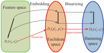
To simulate the real-valued convolutions, we minimize the binary entropy of activations so that the value 2pl(k) - 2u is close to either -1 or 1. Actually, the Hamming distance between two samples xiL and xjL in the final representation can also be simulated using the De(piL, pjL) in the stage of training. Fig. 3 shows the relationships between the original space, the learned Euclidean space and the Hamming space.
4.2 Updating Parameters
As yet, all the optimization problems in the objective Eq. 12 have been addressed. Consequently, our resource-efficient architecture can be easily trained in a similar way of classical methods while the final weights and representations can approximate to the quantized codes. It means the gradient ∂L(F) ∂WL of loss function L(F) w.r.t the filter weights WL could be back propagated to the gradient ∂L(F) ∂W1 in the first layer. However, we have also observed that the gradient would be vanished when some weights are close to the
L }.
| SH-BDNN | SDH | SDHREDHREDH | U-REDHU-REDHUH-BDNN | DB DH | |||||
|---|---|---|---|---|---|---|---|---|---|
| Set | BDNN | BDNN | DH | DH | BDNN | DH | BDNN | DH | DH DH |
| 16bt | 94.2 | 93.3 | 46.8 | 71.6 | 85.4 | 44.2 | 45.6 | 45.4 | 28.243.1 |
| 24bt | 94.4 | 94.1 | - | 72.3 | 88.9 | 45.8 | 49.1 | - | - - |
| 32bt | 95.4 | 94.7 | 51.0 | 74.7 | 90.2 | 48.3 | 52.5 | 47.2 | 32.045.0 |
| 48bt | - | - | - | 76.2 | 91.0 | 49.0 | 55.6 | - | - - |
| 64bt | - | - | 52.5 | 77.9 | 92.4 | 50.3 | 56.2 | - | 44.5 46.7 |
| SH-BDNNDHNSDH*REDHREDH U-REDHU-REDHUH-BDNN DH | DB | |||||||||
|---|---|---|---|---|---|---|---|---|---|---|
| Set | BDNN | DH | DH | DH | BDNN | DH | BDNN | DH | DH | DH |
| 16bt | 65.2 | 59.4 | 18.8 | 49.9 | 55.3 | 19.9 | 23.6 | 17.8 | 16.219.43 | |
| 24bt | 66.2 | 60.3 | - | 51.7 | 56.2 | 22.1 | 25.3 | - | - | - |
| 32bt | 66.5 | 62.1 | 20.8 | 52.2 | 59.5 | 25.6 | 28.9 | 18.5 | 16.624.86 | |
| 48bt | - | - | - | 54.7 | 61.3 | 26.7 | 29.1 | - | - | - |
| 64bt | - | - | 22.5 | 58.1 | 65.7 | 28.8 | 33.1 | - | 17.0 | 27.73 |
quantized codes. To solve this, we use a cumulative gradient to update these weights which are close to the quantized codes. First, in each epoch, we find those weights in Wl using idx = find(log cosh(Wl) < δ). δ is a very small value and Idx is the index of those weights. It is easy to prove that the corresponding items in Wl are close to the quantized codes when the non-negative values are less than a small value. Then, we accumulate these gradients using g(WL, idx) = g(WL, idx) + ∂L(F) ∂Wl (idx). Last, for those weights which have the different signs to the corresponding gradients, we update them using 2g(WL, idx) and set the accumulated gradients to zero. The strategy can make the weights move around the quantized codes.
The detailed algorithm of training binary neural networks for binary embedding is given in Algorithm 1. In the stage of inference, the real-valued weights WL are discarded and only the binary weights B(WL) need to be kept.
5 Experimental Results
We validate our proposed method in two tasks: semantic retrieval and object matching. The common characteristic of these two tasks is that their application in real systems requires efficient prediction and matching. In our method, the balancing parameters λ1 = 0.1, λ2 = 3.5 and λ3 = 125 are fixed in all experiments. Moreover, we use Eq. 10 to capture the special properties of the data. For semantic retrieval tasks, samples can be sampled by category. For the task of object matching, it is possible to select whether the samples belong to the same object or not, according to the correspondence. However, similar to the framework in DH [Liong et al., 2015], we can build our unsupervised version of our proposed badget-aware deep hashing, named as U-REDH, without considering semantic information in Eq. 10. Otherwise, either the triplet loss in Eq. 10 or geometric property in Eq. 11 are considered in REDH. In our model, a deep architecture based on the GoogLeNet [Szegedy et al., 2015] style Inception model is used as the structure of the convolutional neural network. The output layer is replaced by a binarizing layer which is the same as the previous activations in intermediate layers and can produce the required number of binary codes. The parameters will be tuned and updated according to the objective function in Eq. 12 for some specific tasks.
5.1 Semantic Image Retrieval
In this section, CIFAR-10 and MNIST datasets are used to compare our method with the state-of-the-arts. The experimental setting for CIFAR-10 and MNIST, in which label information is provided, is the same as that in [Liong et al., 2015]. Generally, there are two types of dataset partitions and the difference between them that affects MAP performance is the number of gallery. The first setting is the same as the one in DH [Liong et al., 2015], in which, for both datasets, 1000 samples, 100 per class, are randomly selected as the query data, and the remaining samples are used as the gallery set. Whilst, the second setting is the same as the one in BDNN [Do et al., 2016], in which the query set contains 10,000 samples, and the others are treated as gallery set.
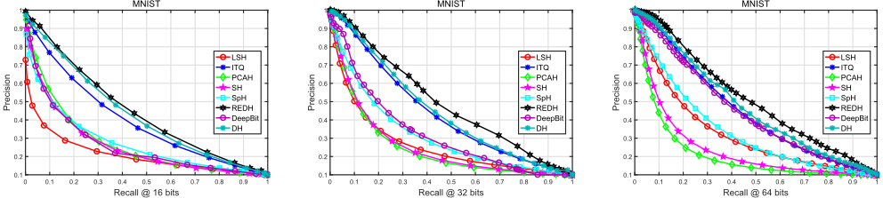
Then the Mean Average Precision (MAP) which is the average precision at the ranks where recall changes, is used to evaluate the overall performance. We also calculate the Precision-Recall curves under varying Hamming distance between the learned binary codes at the code length of 16, 32 and 64, respectively. The deep architecture based hashing methods inclduing DSH [Liu et al., 2016a], DHN [Zhu et al., 2016], DNNH [Lai et al., 2015], BDNN [Do et al., 2016], DH [Liong et al., 2015] and DeepBit [Liny et al., 2016] are used as the baseline methods. Among them, DH [Liong et al., 2015] and DeepBit [Liny et al., 2016] are two unsupervised methods while others are supervised. More five linear unsupervised methods including LSH [Indyk and Motwani, 1998], ITQ [Gong et al., 2013], PCAH [Wang et al., 2012], SH [Weiss et al., 2009], SpH [Heo et al., 2015] and one linear supervised method SDH [Shen et al., 2015] are also compared. Generally, supervised methods use labels to define the sample relationship for guiding the metric learning.
For MNIST dataset, Fig. 4 shows the comparison of Precision-Recall curves between the unsupervised version of REDH and other unsupervised methods in the partition setting of DH [Liong et al., 2015]. We can see that U-REDH can consistently achieve better results than all other non-deep methods and deep architecture-based methods. The comparison results of the overall performance (MAP) between REDH and other supervised and unsupervised deep hashing methods are shown in Table 1. Generally, we can see that the performance using dataset partition of DH [Liong et al., 2015] is lower than that of BDNN [Do et al., 2016] because the former setting has more samples in the gallery set. Moreover, for the task of semantic retrieval, supervised methods perform much better than the unsupervised methods. Unsupervised BDAH outperforms other unsupervised methods. Meanwhile, the performance of supervised BDAH is close to other supervised deep hashing methods, which fully explore the label information to improve the performance. It is worth noting that all other deep hashing methods are real-valued deep architectures and thus, obviously, REDH will run faster and save more memory than them when generating code.
For CIFAR-10 dataset [Krizhevsky and Hinton, 2009], a
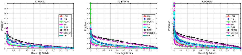
512-D GIST feature vector 2 for each image is taken as the input of models whilst our model directly projects the raw image into binary codes. The compared results on CIFAR10 dataset are given in Table 2 and Fig. 5. The results of all methods on the CIFAR-10 data set are lower than those on the MNIST data set and it means that the retrieval task of real images is harder than that of digital images. We can also observe that label information can boost the performance but the degrees of performance improvement for different methods are varied. Compared with DH, the supervised version of REDH has improved more significantly. It demonstrates that our model can easily incorporate different properties. Overall, we can obtain the same conclusions as the comparison results on MNIST dataset. From Fig. 5, it seems that DeepBit is a little better than unsupervised version of REDH at the length of 16 when the recall rate is above 0.5. In other cases, REDH outperforms other methods on CIFAR-10 dataset.
5.2 Image Matching of the Same Object
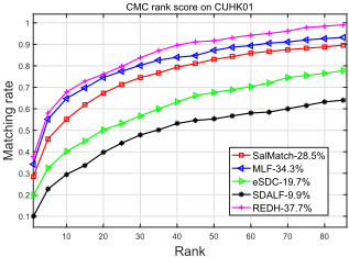
To further validate the proposed method for fast binary embedding, we test it on two matching (re-identification) applications. Hamming distance would be the most efficient measure to compare the samples. Same as most matching methods, Cumulated Matching Characteristics (CMC) [Zhao et al., 2014] curve is used to evaluate the performance.
The first task is to match two images of the same person taken by different cameras. Our model is fine-tuned on the datasets introduced in [Zheng et al., 2015] and then validated on CUHK01 [Zhao et al., 2014] dataset. CUHK01 contains 971 persons, each of which has two images. All the images are normalised to 160 × 60. The experimental setting is the same as [Zhao et al., 2014] where 486 persons are chosen for query and the remaining persons for gallery. Four methods including eSDC [Zhao et al., 2013b], SDALF [Farenzena et al., 2010], SalMatch [Zhao et al., 2013a] and MLF [Zhao et al., 2014] are validated on this dataset. The compared results on CUHK01 dataset are given in Fig. 6. We can see that the proposed method REDH consistently yields better results than the other methods, from 1 to 80 ranks. Actually, only REDH can effectively match the samples in the Hamming space, while other methods use Euclidean distance.
2 Deep features can be used as the input for the classical non-deep learning methods. Performance may increase by about 3%- 10%, but it is still lower than the deep models [Do et al., 2016].
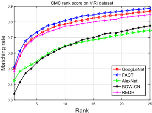
The second task is to match two images of the same vehicle model. VeRi [Liu et al., 2016b] was collected from a real-world urban surveillance scene and contains a total of 776 vehicles captured by 19 cameras. 37, 778 images of the 576 vehicle are used for training while the remaining 13, 257 images of 200 the vehicle are used for the test. Our experiment setup is the same as the original report in [Liu et al., 2016b]. Four methods including GoogLeNet [Szegedy et al., 2015], FACT [Liu et al., 2016b], Bow-CN [van de Weijer et al., 2007] and AlexNet [Krizhevsky et al., 2012] are selected to compare their performance. The compared results on VeRi dataset are given in Fig. 7. FACT, designed for vehicle matching, also uses deep architectures to generate realvalued features. In contrast, REDH learns binary representations through binary networks and runs faster than other methods, including FACT, AlexNet, and GoogLeNet, in the projection and matching phases. In fact, REDH still outperform a real-valued deep architecture: AlexNet. In general, we can see that REDH achieves acceptable results on this dataset.
5.3 Resource-Efficient Analysis
We investigate the memory consumption and the computational time in the stage of code generation. Three general architectures which are popularly used in various applications are compared. Most existing deep hashing methods choose the typical architectures including AlexNet [Krizhevsky et al., 2012], GoogLeNet [Szegedy et al., 2015] and VGG [Simonyan and Zisserman, 2015] as the basic projection function. For example, DeepBit [Liny et al., 2016] uses the VGG16 [Simonyan and Zisserman, 2015] as the basic architecture of deep hashing model. In fact, both memory and calculation depend not only on the number of parameters, but also on the way how it is calculated. In this paper, we resort to change the way of calculation by replacing the multiplications in the convolutional neural networks using the Boolean operations.
The comparison results are given in Table 3. We can see that our model has the same number of parameters as the basic GoogLeNet architecture, but the memory requirement is greatly reduced because only one bit per parameter is required. Moreover, since the Boolean operation is much faster than the multiplication, the calculation time of the inference is also greatly reduced. In summary, we propose a method that can achieve at least a 32x model compression rate and a
| Architectures | AlexNetGoogLeNetVGG-16DeepBit REDH | ||||
|---|---|---|---|---|---|
| Model size | 60M | 5M | 138M | 138M | 5M |
| Memory | 240M | 20M | 552M | 552M | 0.625M |
| Computation (s) | 0.090 | 0.106 | 0.923 | 0.923 | 0.002 |
45x efficiency increase rate.
6 Conclusion
In this paper, we introduce a novel framework to achieve the resource-efficient deep hashing. The model can be easily trained using the classical stochastic gradient descend method because the quantization loss between the quantized values and the learned real-valued weights is minimized. This also leads to a quantized model that is as close to the original trained model as possible. Extensive experiments show that the proposed method can achieve competitive results over the state-of-the-art methods but use much fewer resources.
Acknowledgements
H.H. was partially supported by U.S. NSF IIS 1836945, IIS 1836938, DBI 1836866, IIS 1845666, IIS 1852606, IIS 1838627, IIS 1837956.
@inproceedings{ijcai2019p145,
  title     = {Binarized Neural Networks for Resource-Efficient Hashing with Minimizing Quantization Loss},
  author    = {Zheng, Feng and Deng, Cheng and Huang, Heng},
  booktitle = {Proceedings of the Twenty-Eighth International Joint Conference on
               Artificial Intelligence, {IJCAI-19}},
  publisher = {International Joint Conferences on Artificial Intelligence Organization},
  editor    = {Sarit Kraus},
  pages     = {1032--1040},
  year      = {2019},
  month     = {8},
  note      = {Main track},
  doi       = {10.24963/ijcai.2019/145},
  url       = {https://doi.org/10.24963/ijcai.2019/145},
}
TY - CPAPER TI - Binarized Neural Networks for Resource-Efficient Hashing with Minimizing Quantization Loss AU - Zheng, Feng AU - Deng, Cheng AU - Huang, Heng T2 - Proceedings of the Twenty-Eighth International Joint Conference on Artificial Intelligence, IJCAI-19 PB - International Joint Conferences on Artificial Intelligence Organization PY - 2019 SP - 1032 EP - 1040 DO - 10.24963/ijcai.2019/145 UR - https://doi.org/10.24963/ijcai.2019/145 ER -Copied
Machine-readable versions of this paper, for tools and AI agents:





