
Capturing Spatial and Temporal Patterns for Facial Landmark Tracking through Adversarial Learning
Proceedings of the Twenty-Eighth International Joint Conference on Artificial Intelligence. Main track. Pages 1010-1017.
https://doi.org/10.24963/ijcai.2019/142
Keywords
- Computer Vision: Biometrics, Face and Gesture Recognition
- Computer Vision: Motion and Tracking
Abstract
The spatial and temporal patterns inherent in facial feature points are crucial for facial landmark tracking, but have not been thoroughly explored yet. In this paper, we propose a novel deep adversarial framework to explore the shape and temporal dependencies from both appearance level and target label level. The proposed deep adversarial framework consists of a deep landmark tracker and a discriminator. The deep landmark tracker is composed of a stacked Hourglass network as well as a convolutional neural network and a long short-term memory network, and thus implicitly capture spatial and temporal patterns from facial appearance for facial landmark tracking. The discriminator is adopted to distinguish the tracked facial landmarks from ground truth ones. It explicitly models shape and temporal dependencies existing in ground truth facial landmarks through another convolutional neural network and another long short-term memory network. The deep landmark tracker and the discriminator compete with each other. Through adversarial learning, the proposed deep adversarial landmark tracking approach leverages inherent spatial and temporal patterns to facilitate facial landmark tracking from both appearance level and target label level. Experimental results on two benchmark databases demonstrate the superiority of the proposed approach to state-of-the-art work.
- [Arjovsky et al., 2017] Martín Arjovsky, Soumith Chin- tala, and Léon Bottou. Wasserstein GAN. CoRR, abs/1701.07875, 2017.
- [Asthana et al., 2014] Akshay Asthana, Stefanos Zafeiriou, Shiyang Cheng, and Maja Pantic. Incremental face align- ment in the wild. In CVPR, pages 1859-1866, 2014.
- [Bulat and Tzimiropoulos, 2017] Adrian Bulat and Georgios Tzimiropoulos. How far are we from solving the 2d & 3d face alignment problem?(and a dataset of 230,000 3d facial landmarks). In ICCV, volume 1, page 4, 2017.
- [Chrysos et al., 2018] Grigorios G Chrysos, Epameinondas Antonakos, Patrick Snape, Akshay Asthana, and Stefanos Zafeiriou. A comprehensive performance evaluation of de- formable face tracking "in-the-wild". IJCV, 126(2-4):198- 232, 2018.
- [Cosar and Cetin, 2011] Serhan Cosar and Mujdat Cetin. A graphical model based solution to the facial feature point tracking problem. Image Vision Comput., 29:335-350, 2011.
- [Gehring et al., 2017] Jonas Gehring, Michael Auli, David Grangier, and Yann Dauphin. A convolutional encoder model for neural machine translation. In ACL, pages 123- 135, 2017.
- [Goodfellow et al., 2014] Ian J. Goodfellow, Jean Pouget- Abadie, Mehdi Mirza, Bing Xu, David Warde-Farley, Sherjil Ozair, Aaron C. Courville, and Yoshua Bengio. Generative adversarial networks. CoRR, abs/1406.2661, 2014.
- [Li et al., 2013] Y. Li, S. Wang, Y. Zhao, and Q. Ji. Si- multaneous facial feature tracking and facial expression recognition. IEEE Transactions on Image Processing, 22(7):2559-2573, 2013.
- [Liu et al., 2018] Hao Liu, Jiwen Lu, Jianjiang Feng, and Jie Zhou. Two-stream transformer networks for video-based face alignment. IEEE transactions on pattern analysis and machine intelligence, 40(11):2546-2554, 2018.
- [Miao et al., 2018] Xin Miao, Xiantong Zhen, Xianglong Liu, Cheng Deng, Vassilis Athitsos, and Heng Huang. Di- rect shape regression networks for end-to-end face align- ment. In CVPR, pages 5040-5049, 2018.
- [Peng et al., 2016] Xi Peng, Rogerio S Feris, Xiaoyu Wang, and Dimitris N Metaxas. A recurrent encoder-decoder net- work for sequential face alignment. In ECCV, pages 38- 56, 2016.
- [Sagonas et al., 2016] Christos Sagonas, Epameinondas An- tonakos, Georgios Tzimiropoulos, Stefanos Zafeiriou, and Maja Pantic. 300 faces in-the-wild challenge: Database and results. Image and vision computing, 47:3-18, 2016.
- [Sainath et al., 2015] Tara N Sainath, Oriol Vinyals, An- drew Senior, and Has ¸im Sak. Convolutional, long short- term memory, fully connected deep neural networks. In ICASSP, pages 4580-4584, 2015.
- [Shen et al., 2015] Jie Shen, Stefanos Zafeiriou, Grigoris G Chrysos, Jean Kossaifi, Georgios Tzimiropoulos, and Maja Pantic. The first facial landmark tracking in-the-wild challenge: Benchmark and results. In ICCV Workshops, pages 50-58, 2015.
- [Simonyan and Zisserman, 2014] Karen Simonyan and An- drew Zisserman. Two-stream convolutional networks for action recognition in videos. In NIPS, pages 568-576, 2014.
- [Tai et al., 2019] Ying Tai, Yicong Liang, Xiaoming Liu, Lei Duan, Jilin Li, Chengjie Wang, Feiyue Huang, and Yu Chen. Towards highly accurate and stable face align- ment for high-resolution videos. AAAI, 2019.
- [Wu and Ji, 2015] Yue Wu and Qiang Ji. Shape augmented regression method for face alignment. In ICCV Workshop, pages 979-985, 2015.
- [Wu and Ji, 2019] Yue Wu and Qiang Ji. Facial landmark detection: A literature survey. International Journal of Computer Vision, 127(2):115-142, 2019.
- [Wu et al., 2013] Yue Wu, Zuoguan Wang, and Qiang Ji. Fa- cial feature tracking under varying facial expressions and face poses based on restricted boltzmann machines. In CVPR, pages 3452-3459, 2013.
- [Xiao et al., 2015] Shengtao Xiao, Shuicheng Yan, and Ashraf A. Kassim. Facial landmark detection via progres- sive initialization. In ICCV Workshops 2015, pages 986- 993, 2015.
- [Xiong and De la Torre, 2013] Xuehan Xiong and Fernando De la Torre. Supervised descent method and its applica- tions to face alignment. In CVPR, pages 532-539, 2013.
- [Zhang et al., 2016] Zhanpeng Zhang, Ping Luo, Chen Change Loy, and Xiaoou Tang. Learning deep representation for face alignment with auxiliary attributes. IEEE transactions on pattern analysis and machine intelligence, 38(5):918-930, 2016.
- [Zhu et al., 2015] Shizhan Zhu, Cheng Li, Chen Change Loy, and Xiaoou Tang. Face alignment by coarse-to-fine shape searching. In CVPR, pages 4998- 5006, 2015.
References were extracted automatically from the PDF and may contain errors.
Full text extracted automatically from the PDF; figures, tables and equations may differ. The PDF is the version of record.
1 Introduction
Face alignment, which aims to locate facial landmarks from facial images or videos, has attracted increasing attention and achieved great progress in the past several decades. A comprehensive survey on facial landmark detection can be found in Wu and Ji [2019] and Chrysos et al. [2018].
"In the wild" face alignment is very challenging due to variations in imaging conditions and the diversity inherent in facial appearances. Unlike facial landmark detection, which detects facial feature points from static facial images, facial landmark tracking localizes facial feature points from dynamic facial videos. This task is more complex, since facial videos record spatial changes of appearance as well as temporal dependencies between facial images.
∗Dr. Shangfei Wang is the corresponding author
Current works on landmark tracking can be classified into three categories: a landmark detection approach, an approach modeling spatial and temporal patterns implicitly, and an approach modeling spatial and temporal patterns explicitly. The first approach is tracking by detection, where facial landmark detection is adopted on each frame. Methods in this category, such as Face Alignment Network (FAN) [Bulat and Tzimiropoulos, 2017], are sub-optimal as they ignore temporal dependencies among consecutive frames. The second approach implicitly captures spatial and temporal patterns through time-series models, such as a convolutional neural network (CNN) or a recurrent neural network (RNN). For example, Peng et al. [2016] proposed Recurrent EncoderDecoder Network (REDnet), which encodes temporal information and conducts coarse-to-fine face alignment by RNN structures. Simonyan and Zisserman [2014] proposed TwoStream Convolutional Network (TSCN), in which one CNN extracts spatial patterns from each frame, and a second CNN captures the temporal patterns present in the multi-frame dense optical flow. Liu et al. [2018] proposed Two-Stream Transformer Network (TSTN), which predicts the landmark coordinate residuals using two networks. A CNN structure captures spatial information from cropped shape-index local patches, and an encoder-decoder model integrates temporal dependencies from adjacent frames. These works successfully leverage spatial and temporal patterns in facial appearance, but fail to explore shape and dynamic patterns embedded in ground truth facial feature points, which could be used as further constraints to boost the performance of landmark tracking.
The third approach captures spatial and temporal patterns explicitly by adding manually designed constraints or using probabilistic graphical models. Wu and Ji [2015] proposed a Shape Augmented Regression (SAR) method by adding manually designed global facial shape features into cascaded regression. Tai et al. [2019] proposed a stabilization model (STA) to constrain time delay and deformation smoothness using two loss functions. Although the proposed constraints can reflect specific forms of spatial or temporal dependencies, they fail to consider all spatial and temporal dependencies embedded in ground truth landmarks. Instead of exploiting certain kinds of shape and temporal dependencies, some probabilistic graphic model-based methods model joint label distribution from ground truth landmarks. For example, Wu et al. [2013] proposed an Restricted Boltzmann Machine (RBM) based facial shape model, which is robust to various head poses. Cosar and Cetin [2011] proposed a Markov Random Field (MRF) model, and Li et al. [2013] proposed a Dynamic Bayesian Network (DBN) to capture the spatial and temporal coherence among adjacent frames for facial feature tracking. Probabilistic graphic model-based methods assume an explicit form of joint distribution. These explicit forms of joint label distribution may not be consistent with the ground truth landmark distributions.
To address this, we propose an adversarial learning framework to close the joint distribution inherent in predicted and ground truth facial landmarks. This technique has two advantages. First, under such a framework, the spatial and temporal dependencies embedded in ground truth landmarks are extracted directly from the original labels, with a more diversity than the manually designed constraints. Second, these dependencies are modeled by a deep neural network, i.e., the discriminator, which requires no assumptions of distribution form.
The proposed deep adversarial framework consists of a deep landmark tracker and a discriminator. The deep landmark tracker learns to predict landmark positions from facial image sequences, and tries to fool the discriminator, while the discriminator is adopted to distinguish the tracked facial landmark sequence from the ground truth one. The former implicitly captures spatial and temporal patterns from facial appearance, and the latter explicitly models shape and temporal dependencies existing in ground truth facial landmarks. Due to the complementary capabilities of CNN and RNN in sequence modeling [Sainath et al., 2015; Gehring et al., 2017], both the tracker and the discriminator consist of a combination of CNN and RNN. Through adversarial learning, the proposed deep adversarial landmark tracking network can thoroughly explore facial shape and dynamic models from both appearance and label levels. To the best of our knowledge, we are the first to capture the shape and temporal dependencies from both appearance level and target label level for facial landmark tracking. Experimental results on two databases show a performance boost in accuracy and stability over other state-of-the-art methods, thus demonstrating the effectiveness of our proposed method.
2 Problem Statement
Let I1:T = {I1 , ..., It , ..., IT } be a facial video with T continuous frames, where It ∈ RH×W×3 denotes the RGB facial image of the t th frame with height H and width W. Let gt = (xt∗ 1 , yt∗ 1 , xt∗ 2 , yt∗ 2 , ..., xt∗M , yt∗M ) ∈ R2M be the concatenation of ground truth coordinates for a total of M facial landmarks in It . The ground truths for the whole sequence are denoted by g1:T = {g1 , ..., gt , ..., gT }.
The object of facial landmark tracking is to infer g1:T given I1:T , i.e., to find a function G to map a facial image sequence to a coordinate sequence, as shown in Eq. (1):
3 Methodology
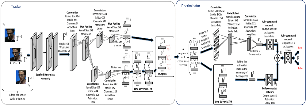
The framework of the proposed approach consists of two deep neural networks, i.e., a tracker and a discriminator, as shown in Fig. 1. The tracker is used to track landmarks from a facial video. The discriminator is introduced to distinguish the predicted landmark positions from the ground truth ones. The tracker tries to confuse the discriminator by predicting landmark positions with joint distributions that are close to the ground truth ones. Through adversarial learning, the inherent spatial and temporal dependencies of a facial sequence are captured from both appearance level and target level for landmark tracking. To facilitate the processing of a long video, we segment it into several short video slices and let the tracker and the discriminator process them in a slice-by-slice way. In order to capture long term dependencies in a video, we design a temporal delivery strategy from slice to slice for both the tracker and discriminator. The proposed deep adversarial landmark tracking network is learned by minimizing a weighted combination of a supervised regression loss and an adversarial loss.
3.1 Tracker
The deep landmark tracker learns to predict landmark positions from facial appearance. As depicted in the left part of Fig. 1, the tracker takes a facial sequence with several adjacent frames as the input, and yields a corresponding sequence of landmark coordinates. Specifically, each facial frame is first processed separately by a stacked Hourglass network with hierarchical parallel and multi-scale blocks, as used in FAN [Bulat and Tzimiropoulos, 2017]. This produces a high-dimensional feature tensor, denoted as Ft , as the representation for the current facial frame. Instead of conducting Heatmap Regression on Ft as Bulat and Tzimiropoulos [2017] did which generates rounding coordinates and may cause quantization errors, we use a CNN to compress Ft into a continuous coordinate vector and a feature vector, i.e, st and ft , where st is the landmark coordinate detected on the current frame and ft is a feature used for temporal integration.
We choose LSTM to integrate temporal information. In the tracker, the LSTM has two layers. The first layer takes the sequence of feature vectors f1 , ..., ft , ..., fT produced by the CNN as input and generates a sequence of hidden states denoted as h11 , ..., ht1 , ..., hT1 , which are the input for the second layer generating another sequence of hidden states denoted as h12 , ..., ht2 , ..., hT2 . These output hidden states are regarded as another sequence of landmark coordinates, which integrate temporal information. And we scale up these hidden states by multiplying them with the length of side of the facial image to cover coordinates on the whole image. The final output of the tracker at the t th frame, i.e., ct , is a weighted average of st and ht2 as follows:
where ct ∈ R2M , which is the concatenation of all M predicted landmark coordinates. γ is the weight coefficient of ht2 .
3.2 Discriminator
The output of the tracker is used as the input for the discriminator, which distinguishes it from ground truth labels as depicted in the right part of Fig. 1. In other words, the discriminator tries to classify the ground truth positions g1:T = {g1 , ..., gt , ..., gT } as "real", and the output of the tracker c1:T = {c1 , ..., ct , ..., cT } as "fake".
We propose a novel structure combining CNN and LSTM to embed and fuse spatial and temporal information in the landmark sequence. For the CNN, g1:T or c1:T is stacked as a matrix with the size of T ×2M, then encoded and compressed by several convolutional layers and flattened to a feature vector denoted as vc. For the LSTM, it takes g1 , ..., gt , ..., gT (or c1 , ..., ct , ..., cT ) as the input and generates a sequence of hidden states denoted as h1 , ..., hT . We choose hT , i.e., the hidden state of the last time step with a summary of the whole sequence, as the output feature for the LSTM module. The output vectors of CNN and LSTM, i.e., vc and hT , are then converted to two vectors of the same size, i.e., uc and ul, by a fully connected network. Based on uc and ul, the features from CNN and LSTM are fused by a weighted average, formulated as:
where λ is a hyper-parameter. Another fully-connected network converts the feature vector u to a scalar denoted as p, which is the final output of the discriminator. p represents the confidence that the input of the discriminator is a "real" sample.
3.3 Temporal Delivery Strategy
For a long video, the tracker and the discriminator process a slice of T consecutive frames at a time, then move to the next slice, if the video does not end. When processing a video slice, we want to not only integrate the temporal information in the current T frames, but also keep a memory from all previous frames of the video to capture long term dependencies. This can be achieved by delivering the temporal information saved in LSTM from the current T frames to the next T frames of the video. Specifically, as the current T frames are processed, the LSTM generates a sequence of memory states and hidden states, denoted as m1 , ...,mT and h1 , ..., hT respectively. We use the memory and hidden state generated in the last time step, i.e., mT and hT , as the initialization states for LSTM when processing the next T frames of the video. We adopt this temporal delivery strategy for the LSTMs in both the tracker and discriminator, so they can capture long-term dependencies in a video.
3.4 Supervised Regression Loss
Face alignment can be performed using the supervised regression method, which trains the tracker G by minimizing the error between the prediction of G and the ground truth, as shown in Eq. (4):
where θG denotes the parameters in G.
3.5 Adversarial Loss
An adversarial learning mechanism is used to capture spatial and temporal patterns from the target label level. The discriminator D tries to distinguish the outputs of the tracker G from ground truth landmarks. The tracker G tries to confuse the discriminator D by making its prediction closer to the ground truth in joint distribution until they are indistinguishable. According to Arjovsky et al. [2017] and Goodfellow et al. [2014], this min-max game can be optimized by the following adversarial loss:
where θD denotes the parameters in D.
3.6 Overall Loss
Our learning framework is a combination of supervised regression and adversarial learning. The overall loss function Lo is a weighted aggregation of Lsup and Ladv, which is shown as follows:
where α and β are two hyper-parameters.
3.7 Training Algorithm
Eq. (6) is used to design the training algorithm, as shown in Alg. 1. Both landmark annotated facial videos and static facial images are used during training.
For training on videos, the first and second term of Eq. (6), i.e., α · Lsup and β · Ladv, are optimized alternately with corresponding procedures, as shown in lines 8-9, 11-12 and 14-15 of Alg. 1. Probability threshold r is used to alternately optimize the tracker or the discriminator by the adversarial loss, as shown in line 10 of Alg. 1. Following Arjovsky et al. [2017], a weight clipping strategy is used to force convergence when updating the discriminator, as shown in line 16 of Alg. 1. The temporal delivery strategy outlined in Section 3.3 captures long-term dependencies in a video, depicted in line 21 of Alg. 1.
For training on images, since these images do not provide any temporal information, we only use them to train the tracker according to the supervised regression loss discarding the LSTM module by assigning γ = 0.0 in Eq. (2), as shown in line 26 fromAlg. 1.
4 Experiments
4.1 Experimental Conditions
We evaluate the proposed method on the 300 Videos in the Wild (300VW) [Shen et al., 2015] dataset and the Talking Face (TF) 1 dataset.
The 300VW dataset is the most popular in-the-wild video dataset for facial landmark tracking. It contains 114 videos with annotated 68 landmarks per image. Each video lasts around one minute with 25-30 frames per second. The benchmark divides 50 videos for training and 64 videos for testing. The testing set is further divided into three categories according to difficulty: well-lit (Scenario 1), mild unconstrained (Scenario 2) and challenging (Scenario 3).
The TF dataset is another video dataset which contains one video from one talking subject. This video contains 5000 frames, and each frame is annotated with 68 landmarks. The landmark definition of the TF is different from the 300VW dataset, so we follow previous works [Liu et al., 2018; Peng et al., 2016] and use seven landmarks common to both datasets for testing.
Following Liu et al. [2018], for experiments on the 300VW dataset, the training set consists of the official training set in the 300VW and 300 faces in the Wild (300W) [Sagonas et
1 [FGNET, 2014] FGNET. Talking face video. [Online]. Avilable: http://www-prima.inrialpes.fr/FGnet/data/01TalkingFace/talking face.html, 2014.
Algorithm 1 Training algorithm
- Input: Landmark annotated facial videos and images Hyper-Parameters: α, β, γ, λ, T, η, r, s Output: θG, θD 1: repeat 2: /***below: training on videos***/ 3: k ←generate a random index from training video list 4: Vk ← the training video with index k 5: if Vk has not been explored before then 6: uk ← the first T frames of Vk 7: end if 8: gθG ←∇θG α · Lsup(uk; θG) 9: θG ← θG - η · Adam(θG, gθG ) 10: if p ∼ uniform(0, 1.0) < r then 11: gθG ← ∇θG β · Ladv(uk; θG, θD) 12: θG ← θG - η · RMSP rop(θG, gθG ) 13: else 14: gθD ← -∇θD β · Ladv(uk; θG, θD) 15: θD ← θD - η · RMSP rop(θD, gθD ) 16: θD ← clip(θD, -s, s) 17: end if 18: if uk is the last T frames of Vk then 19: uk ← the first T frames of Vk 20: else 21: saving the generated memory and hidden states of LSTMs as initialization for processing the next T frames of Vk 22: uk ← the next T frames of Vk 23: end if 24: /***below: training on images***/ 25: ib ← randomly select a batch of training images 26: gθG ←∇θG α · Lsup(ib; θG)|γ=0.0 27: θG ← θG - η · Adam(θG, gθG ) 28: until convergence
al., 2016] dataset. The 300W dataset is an image dataset for landmark detection containing 3,148 training images. For experiments on the TF dataset, since the TF dataset only consists of one video, we just train the proposed method on the 300VW dataset and test it on the TF dataset.
The training videos are taken from the 300VW training set. When testing on the 300VW testing set, the training images are taken from a mixture of all images in the 300W and all frames in the 300VW training set. When testing on the TF dataset, the training images are taken from the 300VW training set only. These images are mixed and shuffled thoroughly before training. All faces are cropped from the detection bounding boxes and resized to 256 × 256 pixels, then fed into the network for training, as Tai et al. [2019] did.
We conduct 10-fold cross validation on the 300VW training set for parameter selection. All hyper-parameters are determined, i.e., α = 0.95, β = 0.45, γ = 0.625, λ = 0.75, T = 20, η = 0.0001, r = 0.2, s = 0.03. After cross validation, hyper-parameters are adopted to re-train the proposed method on the whole training set.
The proposed method is evaluated on both accuracy and stability. Accuracy measures how close the predicted landmark positions are to the ground truth ones. Normalized Root Mean Squared Error (NRMSE) and detection rate are the accuracy metrics utilized. Formulas to calculate these metrics can be found in Shen et al. [2015] and Wu and Ji [2015], respectively. Stability reflects the consistency between the movements of predicted landmarks and ground truths. We use the stability metric adopted by Tai et al. [2019]. A lower NRMSE and a higher detection rate indicate better accuracy; a lower value of the stability metric indicates better stability. During experiments, all hyper-parameters are the default optimal values found by cross validation except for the hyperparameters needing further study.
4.2 Experimental Results and Analyses
In this section, we first make empirical study on the proposed method through different hyper-parameter settings. Due to the limited space, we use NRMSE for illustrating the performance. Then, we make comparison with related work, based on NRMSE, detection rate and the stability metric.
Evaluation for the Output Structure of the Tracker
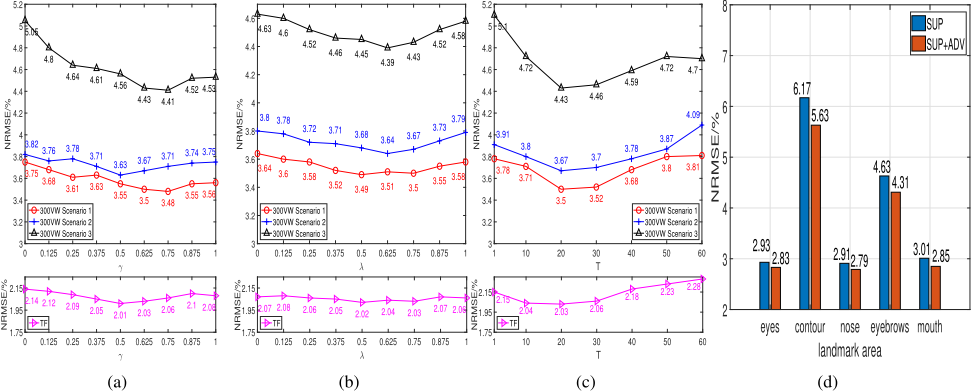
According to Eq. (2), the coordinate prediction of the tracker, i.e., ct , is a weighted average of the landmark coordinate detected on the current frame (st ) and the coordinate generated by the LSTM which integrates temporal information (ht2 ). When γ is 0.0, ht2 is discarded and no temporal information is utilized. As γ increases, the weight of ht2 increases and more temporal information is utilized. NRMSE on the 300VW and TF dataset with different γ are shown in Fig. 2a. When γ is 0.625, which is the optimal value found by 10-fold cross validation, NRMSE decreases by 6.67%, 3.93%, 12.27% and 5.14% on the Scenario 1, 2, 3 of the 300VW dataset and the TF dataset respectively, compared to the setting when γ is 0.0 (ct = st ). NRMSE decreases by 1.69%, 2.13%, 2.21%
and 2.40% on the three scenarios and the TF dataset respectively, compared to the setting when γ is 1.0 ( ct = ht2 ). This demonstrates that the output structure of the adopted tracker is adept at balancing the information from the current frame and the sequential dependencies, improving the performance of landmark tracking.
Evaluation for the Complementary of CNN and LSTM in the Discriminator
According to Eq. (3), the discriminator is a combination of CNN and LSTM weighted by λ. NRMSE on the 300VW and TF dataset with different λ are shown in Fig. 2b. When λ is 0.75, which is the optimal value found by validation, NRMSE decreases by 3.85%, 3.42%, 4.32% and 1.93% on the 300VW Scenario 1, 2, 3 and the TF dataset respectively against using CNN only (λ = 0.0); NRMSE decreases by 2.23%, 3.17%, 3.28% and 1.46% on the three scenarios and the TF dataset respectively against using LSTM only (λ = 1.0). These results demonstrate that CNN and LSTM can complement to each other through a proper combination to compose a good discriminator for adversarial sequential learning.
Evaluation for the Effect of Temporal Length
The proposed method processes T consecutive frames of a video at a time, then move to the next T frames. We evaluate the effect of T on landmark tracking performance in Fig. 2c. When T is 1, there is no sequence information utilized. With the increasing of T, the input sequence is longer and deliveries more temporal information. We find that when T is 20, which is the optimal value found by cross validation, NRMSE decreases by 7.41%, 6.14%, 13.13% and 5.58% on the 300VW Scenario 1, 2, 3 and the TF dataset respectively, compared to the setting when T is 1. However, when T is too large, e.g., T = 60, performance is poorer. This could be because the input becomes more complex as T increases, and the network approaches the ceiling of modeling capability.
| Dataset | SDM | TSCN | CFSS | TCDCN | FAN | TSTN | DSRN | FHR | FHR+STA | Ours |
|---|---|---|---|---|---|---|---|---|---|---|
| 300VWScenario 1 | 7.41 | 12.54 | 7.68 | 7.66 | 5.58 | 5.36 | 5.33 | 4.82 | 4.21 | 3.50 |
| 300VWScenario 2 | 6.18 | 7.25 | 6.42 | 6.77 | 4.87 | 4.51 | 4.92 | 4.23 | 4.02 | 3.67 |
| 300VWScenario 3 | 13.04 | 13.13 | 13.67 | 14.98 | 7.75 | 12.84 | 8.85 | 7.09 | 5.64 | 4.43 |
| Dataset | SDM | CFAN | CFSS | IFA | REDnet | FAN | TSTN | FHR | FHR+STA | Ours |
| TF | 4.01 | 3.52 | 2.36 | 3.45 | 3.32 | 2.31 | 2.13 | 2.07 | 2.10 | 2.03 |
| Dataset | SAR | Ours |
|---|---|---|
| 300VWScenario 1 | 75.30% | 92.45% |
| 300VWScenario 2 | 83.47% | 95.13% |
| 300VWScenario 3 | 52.78% | 91.66% |
| TF | - | 99.12% |
Ablation Study for Adversarial Learning
In this section, we conduct an ablation study for adversarial learning. Two training settings are compared. In the first setting, adversarial learning is discarded from the proposed method by assigning β as 0.0 in Eq. (6). Thus, the tracker is only trained by the supervised regression loss, and this setting is denoted as SUP. For the second one, we keep the adversarial term by setting β as the optimal value (0.45) selected by cross validation. Under such a setting, the whole model, i.e., the tracker and the discriminator, is trained through a combination of the supervised regression loss and adversarial loss. This setting is denoted as SUP+ADV. To further study the effect of adversarial learning, we gather all testing samples from the 300VW dataset and group their landmarks into five facial areas, i.e., eyes, contour, nose , eyebrows and mouth. We just make comparisons on the 300VW dataset, since only seven landmarks are considered in the TF dataset, and the number of landmarks in each area is too small. NRMSE in five areas are shown in Fig. 2d. From Fig. 2d, we can find that adversarial learning improves performance for all facial areas. Contour and eyebrows are the most challenging areas with the highest NRMSE, which is consistent with the observations from Xiao et al. [2015]. Adversarial learning brings the highest NRMSE decrease in these challenging areas, i.e., 8.75% for contour and 6.91% for eyebrows, against eyes (3.41%), nose (4.12%), and mouth (5.32%). These performance improvements are owed to the inherent spatial and temporal patterns captured by adversarial learning.
Comparison with Related Work
This section compares the proposed facial landmark tracking method with state-of-the-art methods, including SDM [Xiong and De la Torre, 2013], TSCN [Simonyan and Zisserman, 2014], IFA [Asthana et al., 2014], CFSS [Zhu et al., 2015], SAR [Wu and Ji, 2015], TCDCN [Zhang et al., 2016], REDnet [Peng et al., 2016], FAN [Bulat and Tzimiropoulos, 2017], TSTN [Liu et al., 2018], DSRN [Miao et al., 2018], FHR and STA [Tai et al., 2019].
| Dataset | FHR | FHR+STA | Ours |
|---|---|---|---|
| 300VWScenario 1 | 2.67 | 1.58 | 0.89 |
| 300VWScenario 2 | 1.77 | 1.09 | 0.84 |
| 300VWScenario 3 | 4.43 | 2.62 | 1.82 |
| TF | 0.97 | 0.69 | 0.59 |
Table 1, 2, 3 and 4 list the experimental results on the 300VW dataset and the TF dataset measured by NRSME, detection rate and the stability metric, respectively. All the experimental results of previous works are copied from Liu et al. [2018], Wu and Ji [2015] and Miao et al. [2018] directly, except for those of FAN, FHR, and FHR+STA. Since their training conditions are different from ours, we re-implement these methods and re-conduct experiments using our training set. Some open source codes 2 are used to facilitate reimplementation.
Compared to FAN, the proposed method decreases NRMSE by 37.27%, 24.64%, 42.84% and 12.12% on the 300VW Scenario 1, 2, 3 and the TF dataset respectively. The improvement may be caused by two factors. First, FAN detects landmark positions on the current frame while ignoring temporal information. Our method captures both spatial and temporal dependencies for facial landmark tracking. Second, FAN may be susceptible to rounding errors caused by heatmap regression. Our method compresses the highdimensional output from the Hourglass into continuous coordinates, avoiding this error.
Our method outperforms significantly REDnet, TSCN and TSTN on accuracy. Compared with TSTN, which achieved the best performance among these three methods, our method has a NRMSE decrease of 34.70%, 18.63%, 65.50% and 4.69% on the 300VW Scenario 1, 2, 3 and the TF dataset, respectively. REDnet, TSCN and TSTN capture spatial and temporal dependencies implicitly from appearance features, while our method uses adversarial learning to explore the spatial and temporal patterns from the target label level as well. Therefore, the proposed method achieves better performance.
2 https://github.com/1adrianb/face-alignment, https://github.com/tyshiwo/FHR alignment
Our method achieves better performance than SAR and STA. With respect to accuracy, our method outperforms the detection rate of SAR by 22.78%, 13.97%, 73.66% on the three scenarios of the 300VW dataset. Compared to FHR+STA, which is a face alignment method equipped with STA, our method shows a decrease in NRMSE of 16.86%, 8.71%, 21.45% and 3.33% on the 300VW Scenario 1, 2, 3 and the TF dataset, respectively. Regarding stability, our method outperforms FHR+STA with a decrease of 43.67%, 22.94%, 30.53% and 14.49% on the stability metric for the respective testing datasets. These comparisons illustrate that our method achieves better performance on both accuracy and stability. SAR and STA are methods that use manually designed features or loss to explicitly encode the spatial and temporal dependencies among landmarks. However, the diverse spatial and temporal constraints in real-world faces can hardly be exhausted manually. In contrast, our method directly extracts all spatial and temporal patterns existing in ground truth landmarks through adversarial learning. Thus, our method can capture more diverse dependencies to further improve landmark tracking.
Cosar and Cetin [2011], Wu et al. [2013] and Li et al. [2013] proposed to use probabilistic graphical models to capture the spatial and temporal dependencies for facial landmark tracking. However, there are no published results of these works on the 300VW dataset nor the TF dataset. Since the experimental data they used are beyond our access, we are unable to make a quantitative comparison to them.
5 Conclusion
We propose an adversarial learning framework to explore the shape and temporal dependencies from both appearance level and target label level for facial landmark tracking. We design a tracker as well as a discriminator with advanced network structures. The former learns to track facial landmarks by capturing spatial and temporal patterns from facial videos, and the latter distinguishes the landmark sequence tracked by the former from the ground truth one. Through adversarial learning, the joint distribution inherent in predicted and ground truth facial landmarks are driven to close. Thus, the proposed method models shape and dynamic patterns from target label level. Experiments on the 300VWdataset and the TF dataset demonstrate that the proposed method can fully capture shape and temporal dependencies, and achieves better performance than state-of-the-art work.
Acknowledgements
This work has been supported by the National Key R&D Program of China (2018YFB1307102) and the National Science Foundation of China (917418129).
@inproceedings{ijcai2019p142,
  title     = {Capturing Spatial and Temporal Patterns for Facial Landmark Tracking through Adversarial Learning},
  author    = {Yin, Shi and Wang, Shangfei and Peng, Guozhu and Chen, Xiaoping and Pan, Bowen},
  booktitle = {Proceedings of the Twenty-Eighth International Joint Conference on
               Artificial Intelligence, {IJCAI-19}},
  publisher = {International Joint Conferences on Artificial Intelligence Organization},
  editor    = {Sarit Kraus},
  pages     = {1010--1017},
  year      = {2019},
  month     = {8},
  note      = {Main track},
  doi       = {10.24963/ijcai.2019/142},
  url       = {https://doi.org/10.24963/ijcai.2019/142},
}
TY - CPAPER TI - Capturing Spatial and Temporal Patterns for Facial Landmark Tracking through Adversarial Learning AU - Yin, Shi AU - Wang, Shangfei AU - Peng, Guozhu AU - Chen, Xiaoping AU - Pan, Bowen T2 - Proceedings of the Twenty-Eighth International Joint Conference on Artificial Intelligence, IJCAI-19 PB - International Joint Conferences on Artificial Intelligence Organization PY - 2019 SP - 1010 EP - 1017 DO - 10.24963/ijcai.2019/142 UR - https://doi.org/10.24963/ijcai.2019/142 ER -Copied
Machine-readable versions of this paper, for tools and AI agents:





