
Unchaining the Power of Partial Delete Relaxation, Part II: Finding Plans with Red-Black State Space Search
Proceedings of the Twenty-Seventh International Joint Conference on Artificial Intelligence. Main track. Pages 4750-4756.
https://doi.org/10.24963/ijcai.2018/660
Keywords
- Heuristic Search and Game Playing: Heuristic Search
- Planning and Scheduling: Search in Planning and Scheduling
- Planning and Scheduling: Planning Algorithms
Abstract
Red-black relaxation in classical planning allows to interpolate between delete-relaxed and real planning. Yet the traditional use of relaxations to generate heuristics restricts relaxation usage to tractable fragments. How to actually tap into the red-black relaxation's interpolation power? Prior work has devised red-black state space search (RBS) for intractable red-black planning, and has explored two uses: proving unsolvability, generating seed plans for plan repair. Here, we explore the generation of plans directly through RBS. We design two enhancements to this end: (A) use a known tractable fragment where possible, use RBS for the intractable parts; (B) check RBS state transitions for realizability, spawn relaxation refinements where the check fails. We show the potential merits of both techniques on IPC benchmarks.
- [Bäckström and Nebel, 1995] Christer Bäckström and Bernhard Nebel. Complexity results for SAS + planning. Computational Intelligence, 11(4):625-655, 1995.
- [Bonet and Geffner, 2001] Blai Bonet and Héctor Geffner. Plan- ning as heuristic search. Artificial Intelligence, 129(1-2):5-33, 2001.
- [Coles et al., 2013] Amanda Jane Coles, Andrew Coles, Maria Fox, and Derek Long. A hybrid LP-RPG heuristic for modelling nu- meric resource flows in planning. Journal of Artificial Intelli- gence Research, 46:343-412, 2013.
- [Domshlak et al., 2015] Carmel Domshlak, Jörg Hoffmann, and Michael Katz. Red-black planning: A new systematic approach to partial delete relaxation. Artificial Intelligence, 221:73-114, 2015.
- [Fox and Long, 2001] Maria Fox and Derek Long. Stan4: A hy- brid planning strategy based on subproblem abstraction. The AI Magazine, 22(3):81-84, 2001.
- [Fox et al., 2006] M. Fox, A. E. Gerevini, D. Long, and I. Serina. Plan stability: Replanning versus plan repair. In Derek Long and Stephen Smith, editors, Proceedings of the 16th International Conference on Automated Planning and Scheduling (ICAPS'06), pages 212-221, Ambleside, UK, 2006.
- Morgan Kaufmann. [Gerevini et al., 2003]
- Alfonso Gerevini, Alessandro Saetti, and Ivan Serina. Planning through stochastic local search and tem- poral action graphs. Journal of Artificial Intelligence Research, 20:239-290, 2003.
- [Gnad and Hoffmann, 2015] Daniel Gnad and Jörg Hoffmann. Red-black planning: A new tractability analysis and heuristic function. In Levi Lelis and Roni Stern, editors, Proceedings of the 8th Annual Symposium on Combinatorial Search (SOCS'15). AAAI Press, 2015.
- [Gnad et al., 2016] Daniel Gnad, Marcel Steinmetz, Mathäus Jany, Jörg Hoffmann, Ivan Serina, and Alfonso Gerevini. Partial de- lete relaxation, unchained: On intractable red-black planning and its applications. In Jorge Baier and Adi Botea, editors, Procee- dings of the 9th Annual Symposium on Combinatorial Search (SOCS'16). AAAI Press, 2016.
- [Haslum, 2012] Patrik Haslum. Incremental lower bounds for ad- ditive cost planning problems. In Blai Bonet, Lee McCluskey, José Reinaldo Silva, and Brian Williams, editors, Proceedings of the 22nd International Conference on Automated Planning and Scheduling (ICAPS'12), pages 74-82. AAAI Press, 2012.
- [Helmert and Domshlak, 2009] Malte Helmert and Carmel Domshlak. Landmarks, critical paths and abstractions: What's the difference anyway? In Alfonso Gerevini, Adele Howe, Amedeo Cesta, and Ioannis Refanidis, editors, Proceedings of the 19th International Conference on Automated Planning and Scheduling (ICAPS'09), pages 162-169. AAAI Press, 2009.
- [Helmert and Geffner, 2008] Malte Helmert and Hector Geffner. Unifying the causal graph and additive heuristics. In Jussi Rin- tanen, Bernhard Nebel, J. Christopher Beck, and Eric Hansen, editors, Proceedings of the 18th International Conference on Au- tomated Planning and Scheduling (ICAPS'08), pages 140-147. AAAI Press, 2008.
- [Helmert et al., 2014] Malte Helmert, Patrik Haslum, Jörg Hoff- mann, and Raz Nissim. Merge & shrink abstraction: A method for generating lower bounds in factored state spaces. Journal of the Association for Computing Machinery, 61(3), 2014.
- [Helmert, 2006] Malte Helmert. The Fast Downward planning sy- stem. Journal of Artificial Intelligence Research, 26:191-246, 2006.
- [Helmert, 2009] Malte Helmert. Concise finite-domain representa- tions for PDDL planning tasks. Artificial Intelligence, 173:503- 535, 2009.
- [Hoffmann and Nebel, 2001] Jörg Hoffmann and Bernhard Nebel. The FF planning system: Fast plan generation through heuristic search. Journal of Artificial Intelligence Research, 14:253-302, 2001.
- [Jonsson and Bäckström, 1995] Peter Jonsson and Christer Bäckström. Incremental planning. In European Workshop on Planning, 1995.
- [Katz and Hoffmann, 2013] Michael Katz and Jörg Hoffmann. Red-black relaxed plan heuristics reloaded. In Malte Helmert and Gabriele Röger, editors, Proceedings of the 6th Annual Sym- posium on Combinatorial Search (SOCS'13), pages 105-113. AAAI Press, 2013.
- [Katz and Hoffmann, 2014] Michael Katz and Jörg Hoffmann. Mercury planner: Pushing the limits of partial delete relaxation. In IPC 2014 planner abstracts, pages 43-47, 2014.
- [Katz et al., 2013] Michael Katz, Jörg Hoffmann, and Carmel Domshlak. Red-black relaxed plan heuristics. In Marie desJardins and Michael Littman, editors, Proceedings of the 27th AAAI Conference on Artificial Intelligence (AAAI'13), pa- ges 489-495, Bellevue, WA, USA, July 2013. AAAI Press.
- [Keyder et al., 2014] Emil Keyder, Jörg Hoffmann, and Patrik Has- lum. Improving delete relaxation heuristics through explicitly represented conjunctions. Journal of Artificial Intelligence Rese- arch, 50:487-533, 2014.
- [Richter and Westphal, 2010] Silvia Richter and Matthias Westp- hal. The LAMA planner: Guiding cost-based anytime plan- ning with landmarks. Journal of Artificial Intelligence Research, 39:127-177, 2010.
References were extracted automatically from the PDF and may contain errors.
Full text extracted automatically from the PDF; figures, tables and equations may differ. The PDF is the version of record.
1 Introduction
Relaxations are prominently used in AI Planning for the generation of heuristic functions (e. g. [Bonet and Geffner, 2001; Hoffmann and Nebel, 2001; Helmert and Domshlak, 2009; Helmert et al., 2014]). The delete relaxation in particular has been highly influential. Under this relaxation, state variables accumulate their values rather than switching between them.
The delete relaxation cannot account for having to move to-and-fro, and it ignores resource consumption. Hence there is a lot of work on taking some deletes into account (e. g. [Fox and Long, 2001; Helmert and Geffner, 2008; Haslum, 2012; Coles et al., 2013; Keyder et al., 2014]). Here we consider red-black planning [Domshlak et al., 2015], a partial delete relaxation method that allows to force delete-relaxed plans to behave like real plans in the limit. A subset of ("red") variables take the delete-relaxed semantics, accumulating values, while the remaining ("black") ones retain the true semantics.
The partition into red and black variables is called a painting, and its choice obviously allows to interpolate between delete-relaxed and real planning. Yet for use as a heuristic function, the painting must be chosen so that red-black plan generation is tractable. Prior work therefore restricts the black variables to what we will refer to as ACI, with acyclic causal-graph dependencies and invertible value-transitions.
Acyclic dependencies and invertible value-transitions occur only in small parts of practical planning tasks, so ACI is typically very far from real planning. How can we actually tap into the interpolation power of red-black planning?
We follow up on prior work on this question [Gnad et al., 2016] (Gnad16 in what follows). Gnad16 have shown how to generate red-black plans for arbitrary paintings, via redblack state space search (RBS), a hybrid of forward search and delete-relaxed planning, where every transition contains a local delete-relaxed planning step over the red variables. Gnad16 explored 1) the generation of red-black seed plans for plan repair with LPG [Gerevini et al., 2003; Fox et al., 2006]; and 2) proving planning tasks unsolvable within the red-black relaxation, via an iteration of more and more refined RBS searches (more and more black variables).
Here, we explore the use of RBS for generating plans. This is the natural complement of 2), in what we envision as a redblack relaxation refinement process. The challenge is to make RBS produce real plans early on, with few black variables. We design two enhancements to this end:
- We create synergy between RBS and ACI, by replacing delete-relaxed planning with ACI planning in RBS. This uses ACI where possible (e. g., moving to-and-fro on an invertible road map), and uses RBS where not (e. g., noninvertible resource consumption). We identify a maximally permissive condition on the black-variable dependencies under which this combination is possible.
- We design an adaptive variant of refinement, locally within a single RBS search space where needed. We check every transition s a-→ s′ for realizability of the red parts, i. e., whether the delete-relaxed plan here works in reality. Non-realizable transitions are pruned, and spawn refinement options: red-black planning tasks starting at s, with additional black variables addressing the nonrealizability of s a-→ s′ . The refinement options become search nodes in an overall heuristic search.
We evaluate our techniques on the IPC benchmarks. In overall performance, A) is competitive, while B) often suffers from too many refinement options. Compared to Gnad16's approach 1), A) is better overall, and both A) and B) are highly complementary to 1) per domain. In five domains, our best configurations outperform the state-of-the-art systems LAMA and Mercury by large margins.
2 Preliminaries
We use the finite-domain representation (FDR) framework [B¨ackstr ¨om and Nebel, 1995; Helmert, 2009]. An FDR planning task is a tuple Π = (V, A, I, G). V is a set of variables v, each with a finite domain Dv. A complete assignment to V is a state. I is the initial state, and the goal G is a partial assignment to V . A is a finite set of actions, where each a ∈ A is a triple (prea, effa, ca). The precondition prea and the effect effa are partial assignments to V ; ca ∈ R+0 is the action's cost. We will sometimes refer to variable-value pairs v = d as facts. For a partial assignment p, V(p) denotes the set of variables instantiated by p. For V ′ ⊆ V(p), by p[V ′ ] := p|V ′ we denote the restriction of p to V ′ . An action a is applicable in a state s if s[V(prea)] = prea. The outcome state sJaK is like s except that sJaK(v) = effa(v) for each v ∈ V(effa).
A transition system is a tuple Θ = (S, L, T, s0, SG). S is a set of states. L is a set of labels. T ⊆ S ×L×S is a set of transitions. s0 ∈ S is the start state and SG ⊆ S is the set of goal states. A plan for a state s is a transition path from s to a state in SG. The state space of Π is the transition system ΘΠ where S is the set of states in Π, L = A, (s, a, s′ ) ∈ T iff a is applicable in s and s′ = sJaK, s0 = I, and s ∈ SG if s[V(G)] = G. A plan π for I in ΘΠ is called a plan for Π.
The causal graph (e. g. [Jonsson and B¨ackstr¨om, 1995; Helmert, 2006]) is a digraph with vertices V and an arc (v, v′ ) if v ̸= v′ and there exists an action a ∈ A such that (v, v′ ) ∈ [V(eff(a)) ∪ V(pre(a))] × V(eff(a)).
3 Red-Black Planning
We next give an overview of red-black planning and associated techniques, as needed to understand our contribution.
3.1 Definitions
A red-black planning task, or RB task, is a tuple ΠRB = (V B , V R ,A, I,G) with V B ∩ V R = ∅, where Π := (V,A, I,G) is an FDR task with V := V B ∪ V R . V B is the set of black variables, V R is the set of red variables. States are now RB states sRB , which map each variable v to a subset of its domain, sRB (v) ⊆ Dv, where |sRB (v)| = 1 for v ∈ V B . In the RB initial state sRB 0 each variable v is mapped to {I(v)}. RB goal states are those sRB where G(v) ∈ sRB (v) for all v ∈ V(G). An action a is applicable in an RB state sRB if prea(v) ∈ sRB (v) for all v ∈ V(prea). Upon executing a in sRB , v ∈ V(effa)∩V B is set to {effa(v)}, and v ∈ V(effa) ∩ V R is set to sRB (v) ∪ {effa(v)}. The outcome state is denoted sRB JaK. A plan πRB under this semantics is an RB plan for ΠRB . We also refer to πRB as an RB plan for Π, viewing ΠRB as a red-black relaxation of Π, where the choice of V B vs. V R is a painting defining the relaxation.
The red-black relaxations of any FDR task Π form a refinement hierarchy, with more refined relaxations having larger sets V B . At the extremes, for V B = V we obtain real planning, and for V B = ∅ we obtain fully delete-relaxed planning.
Example 1. Our example task Π has variables V = {T,M, A, B} with domains DT = {l1, l2}, DM = {0, 1, 2}, DA = {0, 1}, DB = {0, 1}. T encodes a traveling agent with two locations l1 and l2, initially l2. The goal is to be at l2, and to possess each product A and B. Each product is available at l1 at price 1; A is also available at l2, but at price 2. M is the available money. The actions have the form go(l, l′ ) and buy(l, p, m). For example, go(l1, l2) has precondition {T = l1} and effect {T = l2}, and buy(l1, A, 2) has precondition {T = l1, M = 2} and effect {A = 1, M = 1}.
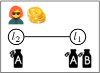
A fully delete-relaxed plan for this task has two flaws: 1) it does not go back from l1 to l2; 2) it may choose to buy A at l2 instead of l1, over-spending the budget. We can fix 1) by painting T black, and we can fix 2) by painting M black. In the red-black relaxation where V B = {T,M} and V R = {A, B}, every RB plan for Π is a real plan for Π.
3.2 Tractable Fragment: ACI
The initial line of work on red-black planning [Domshlak et al., 2015], culminating in the Mercury system's success at IPC'14 [Katz and Hoffmann, 2014], generates a heuristic function based on the tractable fragment ACI. We simplify some details in what follows, for easier exposition.
ACI requires 1) that the causal graph over the black variables is acyclic, and 2) that every black variable is invertible. A variable v is invertible if every value transition can be inverted under the same (or easier) conditions on other variables. An RB plan can then be generated by finding a fully delete-relaxed plan π+, and running ACI plan repair on π+ to obtain an RB plan πRB . The repair process executes π+ step-by-step under the red-black semantics; whenever a condition (precondition or goal) g on V B is not satisfied, the process inserts a subsequence π achieving g. The latter is always possible, in time polynomial in the length of π: thanks to 1), V B can be solved in a sequence from clients (variables which can only be modified through actions depending other variables) to servants (the dependent variables); thanks to 2), whenever a servant v must provide a value d ∈ Dv for a client, v can reach d from its current value. 1
Example 2. In Example 1, T is invertible. A relaxed plan is π+ = 〈buy(l2,A, 2), go(l2, l1), buy(l1,B, 2)〉. ACI plan repair with V B = {T} finds flaw 1), π+ does not satisfy the goal T = l2. It inserts go(l1, l2) at the end to fix that.
Given an FDR task Π, the painting strategies associated with ACI choose V R so as to guarantee that the resulting relaxed task ΠRB is in ACI. A major weakness in practice here is the restriction of V B to invertible variables. In our example, T is the only such variable; we cannot paint M black, so we cannot fix flaw 2) pertaining to money consumption.
Intuitively, using ACI instead of full delete relaxation fixes the "moving to-and-fro" issue, for invertible moves now painted black (here: T). But it does not address resource consumption, which involves non-invertible variables (here: M).
3.3 Red-Black State Space Search
To enable convergence to real planning in the limit, red-black planning methods are required that can handle arbitrary paintings. Addressing this, Gnad et al. [2016] (Gnad16) have introduced red-black state space search (RBS). RBS performs forward search with a relaxed fixed point over the red variables at each transition. At plan extraction time, RBS augments the solution path with a relaxed plan at each transition.
1 In our implementation, we adapted red facts following, the more advanced repair algorithm by Katz and Hoffmann [2013].
We require some notations. The red actions in an RB state sRB , denoted AR (sRB ), are the actions available to the relaxed fixed point at sRB : the actions that comply with the blackvariable values. AR (sRB ) := {aR | a ∈ A, prea[V B ] ⊆ sRB , effa[V B ] ⊆ sRB }, where aR is the projection of a onto V R .
The relaxed fixed point at sRB is now formalized in terms of a local planning task, namely the RB task Π+(sRB ) := (∅, V R , AR (sRB ), sRB [V R ], ∅). The red completion of sRB is the RB state F +(sRB ) where F +(sRB )[V B ] = sRB [V B ], and F +(sRB )[V R ] is the set of all facts reachable in Π+(sRB ).
Definition 1 (Gnad16). Let ΠRB be an RB planning task. The RB state space is the transition system ΘRB = (SRB , T RB , A, sRB 0 , SRB G ). SRB is the set of RB states. sRB 0 is the RB initial state. SRB G = {sRB | F +(sRB ) is RB goal state}. T RB is the set of transitions sRB a-→ tRB where a is applicable to F +(sRB ), eff(a)[V B ] ̸⊆ sRB [V B ], and tRB = F +(sRB )JaK.
Example 3. Setting V B = {M}, F +(sRB 0 ) contains T = l1 and T = l2, but neither A = 1 nor B = 1 as buying a product affects the black variable M. The outgoing transitions of sRB 0 are the buy actions. 〈buy(l1,A, 2), buy(l1,B, 1)〉 leads to an RB goal state. For buy(l2,A, 2), in contrast, the outcome RB state tRB has tRB (M) = {0}, so no further actions are applicable here and we detect that this is a dead-end.
RB plan extraction augments backward solution path extraction with a relaxed plan extraction step at each transition. Assume that π = 〈a0, . . . , an-1〉 is a plan for ΘRB , assume that backward extraction has already extracted an RB plan for the postfix πk := 〈ak, . . . , an-1〉, and assume that the transition taken by ak-1 in π is sRB k-1 ak-1 ---→ sRB k . Then the red goal for relaxed plan extraction at this transition is G(sRB k-1 ) := Regress R (G, ak-1◦πk)\sRB k-1 [V R ], where Regress R is regression in the projection onto V R . Intuitively, G(sRB k-1 ) is the set of red facts that must be achieved before ak-1, and that cannot be achieved further below. Any relaxed plan extraction mechanism can now be used on Π+(sRB k-1 ) to find a relaxed plan π+(sRB k-1 ) achieving G(sRB k-1 ). Then πk is replaced by π+(sRB k-1 ) ◦ ak-1 ◦ πk, and we iterate.
Example 4. In Example 3, denote π = 〈buy(l1,A, 2), buy(l1,B, 1)〉 = 〈a0, a1〉. Denote the RB states along π as sRB 0 , sRB 1 , sRB 2 . Plan extraction first processes sRB 1 a1 -→ sRB 2 . The red goal here is G(sRB 1 ) = ∅, as Regress R ({A = 1,B = 1}, buy(l1,B, 1)) = {T = l1,A = 1} and sRB 1 [V R ] = {T = l2, T = l1,A = 0,A = 1,B = 0}. The postfix thus simply is π1 = 〈buy(l1,B, 1)〉. In the next step though, at sRB 0 a0 -→ sRB 1 , the red goal is G(sRB 0 ) = {T = l1}, leading to the relaxed plan 〈go(l2, l1)〉 and thus to the overall red-black plan πRB = 〈go(l2, l1), buy(l1, A, 2), buy(l1, B, 1)〉.
Observe that πRB in Example 4 is correct about M, but is flawed regarding T (as πRB does not go back from l1 to l2 at the end, leaving the goal T = l2 unsatisfied). This is complementary to the tractable fragment ACI, which can fix T but cannot fix M (cf. Example 2). The first new method we propose here is motivated by this kind of complementarity. We combine RBS with ACI to handle each kind of flaw with the most appropriate method.
4 Combining RBS with ACI
Any flaw in an RB plan πRB can in principle be fixed by painting the respective variable v black, V B := V B ∪ {v}, and re-running RBS. Yet ΘRB grows exponentially in |V B |. Can we avoid the computational cost incurred by painting v black?
As we now show, the answer is yes - if, like for v = T in Example 4, we can handle v by ACI instead. We can use ACI to effectively handle a tractable part of the task at hand (e. g. invertible moves to-and-fro), combined with RBS to handle the remainder (e. g. resource consumption).
4.1 The RBS+ACI Framework
Our combined framework, that we baptize RBS+ACI, distinguishes black variables of two different kinds, handled by RBS vs. ACI. So a painting is now a partition of V into three subsets V RBS , V ACI , V R where V B = V RBS ∪ V ACI .
Assume that such a partition is given. We need an RB plan relative to the entire set V B of black variables, i. e. for the RB task (V RBS ∪ V ACI , V R , A, I, G). The basic idea is to apply ACI plan repair on the outcome of RBS on the coarser (more relaxed) task ΠRB + := (V RBS , V R ∪ V ACI ,A, I,G).
ACI plan repair is defined for fully delete-relaxed plans, not RB plans, so we must adapt the repair process. We must make sure that the repair 1) is always possible given the black part V RBS already fixed, and 2) never affects that fixed part.
Let π be the plan found by RBS for ΠRB + . Our adapted repair process, RBS+ACI plan repair, computes a plan without conflicts on the entire set of black variables V RBS ∪V ACI , fixing unsatisfied conditions only on V ACI without modifying the conflict-free V RBS .
To ensure 2), an obvious and natural requirement is that there is no a ∈ A with V(effa) ∩ V ACI ̸= ∅ and V(effa) ∩ V RBS ̸= ∅. That is, the repair actions will never affect V RBS .
Ensuring 1) is more tricky. In RBS on ΠRB + , the red completion F +(sRB ) of any state sRB uses only actions whose precondition is satisfied given the black variable assignment sRB [V RBS ]. So one may think (and we did think at first) that no further restrictions are needed. However, across transitions sRB a-→ tRB , the fixed repair context changes from sRB [V RBS ] to tRB [V RBS ]. This causes problems because, during RBS, the values reached for V ACI in F +(sRB ) are propagated to tRB . But due to the different context tRB [V RBS ], the repair process at tRB cannot necessarily reach these values.
Similar to Gnad and Hoffmann [2015], we impose that there is no a ∈ A with V(effa) ∩ V ACI ̸= ∅ and V(prea) ∩ V RBS ̸= ∅, i. e., the repair actions do not have preconditions on V RBS . We next show that this restriction is sufficient (the repair will always work). We then show that the restriction is necessary for computational reasons.
The conjunction of our two restrictions is equivalent to the absence of a causal graph arc from V RBS to V ACI . We say in this case that V ACI does not depend on V RBS .
Proposition 1. Given an RB planning task ΠRB = (V B , V R , A, I,G), and a partition of V B into V RBS and V ACI so that (V ACI , V R ∪ V RBS , A, I, G) is in ACI, and V ACI does not depend on V RBS . Let π be an RB plan for ΠRB + = (V RBS , V R ∪ V ACI ,A, I,G). Then RBS+ACI plan repair on π succeeds, and its output πRB is an RB plan for ΠRB .
Proof. Any action a that may be inserted by ACI plan repair, and hence by RBS+ACI plan repair, affects a variable in V ACI . Therefore, by prerequisite, 1) a has no effect on V RBS , and 2) a has no precondition on V RBS . So the arguments given by Katz et al. [2013] remain applicable.
Example 5. Say we set V RBS = {M} and V ACI = {T}. Note that M depends on T : this dependency direction is allowed. RBS is run on ΠRB + = ({M}, {T,A,B},A, I,G). The outcome is π = 〈go(l2, l1), buy(l1,A, 2), buy(l1,B, 1)〉. Running ACI plan repair on π finds the unsatisfied goal condition g = {T = l2} at the end. This is repaired by appending 〈go(l1, l2)〉 to π, yielding a plan for the original task.
Proposition 1 shows that our RBS+ACI framework is sound for RB planning in ΠRB . Completeness holds, too:
Proposition 2. Under the prerequisites of Proposition 1, an RB plan for ΠRB = (V RBS ∪ V ACI , V R , A, I, G) exists iff an RB plan for ΠRB + = (V RBS , V R ∪ V ACI ,A, I,G) exists.
Proof. The "if" direction holds by Proposition 1. The "only if" direction holds because ΠRB is a refinement of ΠRB + .
So our approach works provided there is no CG arc from V RBS to V ACI . Let us show that this restriction is necessary. Consider the decision problem RBS-dependent ACI PlanGen, defined as follows. Given ΠRB = (V B , V R ,A, I,G) and a partition of V B into V RBS and V ACI s.t. (V ACI , V R ∪V RBS , A, I, G) is in ACI, and all CG arcs between V RBS and V ACI , if any, go from V RBS to V ACI . Given an RB plan π for ΠRB + = (V RBS , V R ∪V ACI ,A, I,G). Denote by π|V RBS the subsequence of V RBS -affecting actions in π. Decide whether π|V RBS is a subsequence of an RB plan for ΠRB .
Theorem 1. RBS-dependent ACI PlanGen is NP-hard.
Proof sketch. By reduction from SAT. Our planning encoding contains value-choosing actions for propositional variables pi, and clause-satisfying actions for clauses cj. In the construction, V RBS contains a single "indicator" variable v; V ACI contains variables vpi representing the choice of values; and V R contains variables vcj representing whether a clause has been satisfied yet. Specifically, v has domain {0, 1} and a single action a[v01] moving v from its initial value 0 to 1. We can move vpi invertibly between its initial value u and d ∈ {0, 1}, but under the precondition v = d. Satisfying a clause requires as precondition not only a suitable pi value, but also v = 1. Given this, an RB plan for ΠRB exists iff φ is satisfiable. Yet any RB plan π for ΠRB + has the same V RBS - affecting subsequence π|V RBS = 〈a[v01]〉.
The full proof of Theorem 1 will be made available in an online TR. By the theorem, given the fixed solution path π|V RBS found by RBS for ΠRB + , augmenting π|V RBS to an RB plan for ΠRB is hard. In our framework, such augmentation is done by red (delete-relaxed) planning in ΠRB + alongside
π|V RBS , followed by RBS+ACI plan repair. So one of these steps would need to have worst-case exponential runtime (unless P = NP). In other words, efficient RBS+ACI plan repair is not possible when allowing CG arcs from V RBS to V ACI .
In practice, i. e., in our overall planning algorithm introduced next, one can ameliorate the situation by attempting RBS+ACI plan repair even if V ACI does depend on V RBS . If the repair succeeds, all is fine. We only need to act - remove the problematic variable(s) from V ACI - if the repair fails.
4.2 Overall Planning Process: Iterated RBS+ACI
We now know how to solve any RB task ΠRB with a painting V RBS , V ACI , V R that qualifies for Proposition 1. But our aim here is to find real plans, for the original FDR input task Π. So RBS+ACI becomes a tool within an overall planning process.
That process is a loop around RBS+ACI searches with increasingly refined paintings. In a pre-process, we compute an ACI painting V B 0 , V R 0 using the default painting strategy in Mercury, which orders the variables by causal graph level and iteratively paints variables red until the black CG is a DAG [Katz and Hoffmann, 2014]. We then initialize our painting as V RBS := ∅, V ACI := V B 0 , V R := V R 0 . We run RBS+ACI on that painting. If an RB plan does not exist, we know that Π is unsolvable and we stop. Otherwise, we now have an RB plan πRB . We check whether πRB is a real plan for Π. If yes, we stop. Otherwise, we refine our painting. Namely, we simulate the execution of πRB under the real planning semantics in Π, and we count the number of flaws associated with each variable v ∈ V R . We select v ∈ V R with a maximal number of flaws (a criterion adapted fromMercury). We set V RBS := V RBS ∪ {v} and V R := V R \ {v}, and iterate.
Adding v to V RBS may introduce dependencies of V ACI on V RBS . Therefore, as discussed above, at some point RBS+ACI plan repair may fail. In that case, we move the culprit variable(s) from V ACI to V R , re-establishing the Proposition 1 guarantee that repair will succeed. The red-black relaxation considered is, then, no longer a refinement of the previous one. But convergence to V B = V remains intact, so that the completeness of the overall planning process is preserved.
Whenever checking whether an intermediate RB plan πRB works under the real planning semantics in Π, a variant is to commit to the prefix that works. We will refer to this as prefix-execution. The advantage is that the next iteration of RBS+ACI will not have to start from scratch on the initial state. On the downside, of course this loses completeness.
5 Adaptive Refinement via Realizability
An iterative refinement loop around RBS, as in iterated RBS+ACI, is wasteful in that every iteration of RBS starts from scratch, re-building the entire RB state space. Prefixexecution fixes this, but in a very limited way. Ideally, like other abstraction refinement processes, we ought to refine in an adaptive manner, only where needed, and do so incrementally within a single, iteratively refined, relaxed search space.
But how to do this in RBS, and effectively for the purpose of finding real plans? The straightforward approach would be to search until an RB plan πRB is found, execute πRB against the real semantics until the first flaw occurs at RB state sRB , then accordingly refine the painting and re-do the RBS search space below sRB . But there are a number of issues with this. First, it saves us only the work otherwise done above sRB (similarly as the much simpler prefix-execution). Second, with many black variables - as needed to find real plans - finding πRB becomes very expensive so there will be long time intervals between the local refinement steps. Which is especially wasteful as, third, things often go wrong at the root of an RBS sub-tree already. To illustrate the latter, say that the only action applicable at the root sRB has red preconditions p and q, each of which is reached in F +(sRB ) but which are in conflict so their conjunction is not reachable under the real semantics. Then all search below sRB is wasted.
Given these observations, here we design an eager approach, imposing refinements whenever a transition in ΘRB will not work out in reality. We first show how to do this in RBS, then we discuss the combination with ACI.
5.1 Realizability Refinement: X-RBS
Let sRB be any RB state in ΘRB , and let sRB a-→ tRB be any outgoing transition of sRB . By construction, we know that prea[V R ] ⊆ F +(sRB ). That is, the red preconditions of a can be achieved in the delete-relaxed task Π+(sRB ) at sRB . Let now π+X be a relaxed plan for the goal prea[V R ] in Π+(sRB ), extracted by some relaxed-plan extraction method X. If π+X achieves prea[V R ] under the real semantics V B = V , we say that sRB a-→ tRB is realized by π+X and is realizable given X.
Definition 2. Let ΠRB be an RB planning task, and let X be a relaxed-plan extraction method. The X-RB state space is the transition system ΘRB X defined like ΘRB except that:
- (i) transitions sRB a-→ tRB not realizable given X are pruned;
- (ii) if sRB a-→ tRB is realized by π+X , then tRB is the outcome state of executing π+X ◦ a in sRB with V B = V .
Some remarks are in order. First, the rationale behind (i) is that red-black plans will be extracted using X, so if X does not actually achieve prea in reality then sRB a-→ tRB won't be in a real plan. It is of course a restriction here to commit to X. But there is no systematic alternative: short of a fullscale planning process for prea - giving up on the relaxation altogether - if X does not find a real plan, then the best one could do is try another relaxed plan extraction method X'.
Second, that said, Definition 2 is only one half of the story. Whenever a transition sRB a-→ tRB is pruned by (i), we spawn a refinement option, discussed in detail below. A refinement option is a refined RB planning task at sRB , addressing the reason for non-realizability of sRB a-→ tRB .
Finally, (ii) has the immediate effect that every reachable state sRB in ΘRB X is in fact a real state. It turns the red part of the search (the method X) into a fast macro-generator to the next applicable black-variable affecting action. Observe that this is a natural match with our realizability check. What realizability affirms is that, in reality, we can reach prea at sRB . In contrast, the over-approximated state transition, without (ii), would pretend that we can reach the entire set F +(sRB ). Intuitively, we can check the validity of sRB a-→ tRB only in a limited way, because we don't a-priori know what the red goal might be here at plan extraction time. So we commit to the minimal way of both, checking and using, the transition. (On the side, realizability checks without (ii) would apply the real semantics starting from an RB state, another mismatch.)
Now, that said, (ii) is a choice we made in our work so far. Exploring alternate definitions is a topic for future work.
Let us now turn to refinement options:
Definition 3. Let ΠRB = (V B , V R , A, I, G) be an RB planning task. Let sRB a-→ tRB be a transition pruned in ΘRB X , not realized by π+X . Let v ∈ V R be s.t. π+X contains a maximal number of flaws on v. Then ΠRB +v (sRB ) := (V B ∪ {v}, V R \ {v},A, sRB ,G) is a refinement option for sRB a-→ tRB .
Whenever a transition sRB a-→ tRB is pruned in our exploration of ΘRB X , we generate a refinement option ΠRB +v (sRB ). That option is inserted as a search node into the overall (heuristic) search. Thus, the search decides not only which states to explore, but also which refinement is used to explore that state. We will refer to this overall search framework as X-RBS.
Observe that the under-approximation (ii) loses completeness, i. e., our overall search space may not contain a plan: below realizable transitions, the commitment to π+X may exclude the solutions. As an optional fix, refinement-explored, we also spawn refinement options at nodes sRB all of whose descendants have been unsuccessfully explored. In such a case, we do not have a concrete flaw to fix, so we pick a variable v ∈ V R to paint black arbitrarily.
5.2 Combination with ACI
The number of refinement options can be a major source of computational overhead in X-RBS. One way to ameliorate this is to combine X-RBS with ACI (X-RBS+ACI): replacing delete-relaxed planning with tractable red-black planning will result in fewer flaws, and in more realizable transitions.
The combination is simple in X-RBS as relaxed planning occurs only at individual transitions sRB a-→ tRB . It 1) generates F +(sRB ) to test whether prea is relaxed-reachable; it 2) extracts a relaxed plan using method X, to check realizability.
Using ACI instead, 1) remains unchanged. For 2), we use ACI plan repair on top of X. This uses separate sets V RBS vs. V ACI of black variables as before, but with no constraint on their dependencies: in a realizability check - against the real semantics - a success guarantee cannot be given anyhow.
6 Experiments
Our techniques are implemented on top of Gnad16's RBS, which modifies Fast Downward (FD) [Helmert, 2006] in a minimally intrusive way, exchanging the state and state transition data structures while preserving all search algorithms. All our configurations run FD's greedy best-first dual-queue search with Gnad16's hFF extension and preferred operators.
We run each of RBS and X-RBS with vs. without ACI. We run RBS with vs. without prefix-execution (PE), and X-RBS with vs. without refinement-explored (RE), yielding eight different configurations. Among these, RBS with neither ACI nor prefix-execution is a baseline easily derived from (though not evaluated by) Gnad16. To represent the state of the art in satisficing planning, we run LAMA [Richter and Westphal, 2010] and Mercury [Katz and Hoffmann, 2014]. We also run the best-performing LPG-plan-repair configuration by Gnad16. This paints 90% of the variables black, uses RBS to find an RB plan πRB , then calls LPG to repair πRB into a real plan.
| RBS | X-RBS | ||||||||||
|---|---|---|---|---|---|---|---|---|---|---|---|
| +PE | +ACI +PE | +RE | +ACI +RE | RBS +LPG | LAMA | Mer- cury | |||||
| Airport (50) | 27 | 28 | 27 | 28 | 41 | 43 | 41 | 44 | 42 | 32 | 32 |
| Barman (40) | 0 | 3 | 0 | 3 | 0 | 7 | 0 | 0 | 24 | 39 | 40 |
| Blocks (35) | 35 | 35 | 35 | 35 | 35 | 35 | 24 | 33 | 35 | 35 | |
| Childsnack (20) | 5 | 20 | 9 | 10 | 0 | 0 | 0 | 0 | 4 | 5 | 0 |
| Depots (22) | 15 | 17 | 16 | 18 | 1 | 9 | 14 | 15 | 21 | 20 | 21 |
| Driverlog (20) | 19 | 18 | 20 | 19 | 2 | 7 | 3 | 9 | 18 | 20 | 20 |
| Elevat (50) | 45 | 47 | 50 | 50 | 0 | 12 | 50 | 50 | 50 | 50 | 50 |
| Floortile (40) | 3 | 3 | 6 | 7 | 0 | 4 | 0 | 0 | 9 | 8 | 8 |
| Freecell (80) | 71 | 69 | 71 | 69 | 69 | 61 | 69 | 60 | 35 | 79 | 80 |
| GED (20) | 10 | 9 | 10 | 10 | 20 | 20 | 14 | 0 | 4 | 20 | 20 |
| Grid (5) | 4 | 4 | 5 | 4 | 0 | 2 | 4 | 5 | 4 | 5 | 5 |
| Hiking (20) | 20 | 20 | 15 | 17 | 18 | 15 | 18 | 20 | 19 | 18 | 20 |
| Logistics (63) | 62 | 62 | 63 | 63 | 0 | 12 | 63 | 63 | 35 | 63 | 63 |
| Maintenan (20) | 11 | 7 | 11 | 7 | 0 | 0 | 0 | 0 | 0 | 7 | |
| Mprime (35) | 35 | 34 | 35 | 35 | 3 | 18 | 35 | 34 | 35 | 35 | 35 |
| Mystery (19) | 16 | 13 | 17 | 13 | 1 | 8 | 19 | 18 | 16 | 19 | 19 |
| NoMystery (20) | 19 | 19 | 19 | 17 | 0 | 4 | 1 | 4 | 19 | 11 | 14 |
| ParcPrin(50) | 49 | 49 | 49 | 49 | 39 | 48 | 36 | 37 | 35 | 49 | 50 |
| Parking (40) | 12 | 13 | 11 | 13 | 0 | 0 | 0 | 0 | 0 | 40 | 40 |
| Pathways (30) | 21 | 28 | 21 | 28 | 27 | 26 | 27 | 26 | 21 | 23 | 30 |
| PegSol (50) | 50 | 50 | 50 | 50 | 50 | 50 | 50 | 37 | 16 | 50 | 50 |
| PipesNoT (50) | 35 | 38 | 36 | 38 | 34 | 25 | 25 | 17 | 39 | 43 | 44 |
| PipesTank (50) | 31 | 26 | 28 | 30 | 26 | 20 | 34 | 18 | 24 | 42 | 42 |
| PSR (50) | 50 | 50 | 50 | 50 | 0 | 49 | 0 | 49 | 50 | 50 | 50 |
| Rovers (40) | 40 | 40 | 40 | 40 | 2 | 16 | 18 | 20 | 40 | 40 | |
| Satellite (36) | 36 | 36 | 36 | 36 | 0 | 5 | 36 | 36 | 36 | 36 | |
| Scanaly (50) | 42 | 46 | 42 | 50 | 43 | 42 | 44 | 44 | 46 | 50 | 50 |
| Sokoban (50) | 20 | 15 | 22 | 13 | 44 | 44 | 29 | 9 | 5 | 48 | 42 |
| Storage (30) | 18 | 20 | 18 | 18 | 16 | 17 | 28 | 28 | 25 | 19 | 19 |
| Tetris (20) | 0 | 3 | 0 | 2 | 1 | 0 | 3 | 2 | 0 | 13 | 19 |
| Thoughtful (20) | 6 | 11 | 6 | 10 | 15 | 13 | 9 | 5 | 16 | 13 | |
| Tidybot (20) | 8 | 6 | 7 | 8 | 0 | 2 | 0 | 0 | 13 | 17 | 15 |
| TPP (30) | 30 | 30 | 30 | 30 | 0 | 10 | 30 | 27 | 30 | 30 | 30 |
| Transpo (70) | 31 | 33 | 70 | 70 | 0 | 20 | 61 | 57 | 45 | 61 | 70 |
| Trucks (30) | 12 | 12 | 12 | 12 | 4 | 10 | 0 | 8 | 20 | 15 | 19 |
| VisitAll (40) | 3 | 4 | 40 | 40 | 3 | 3 | 40 | 40 | 4 | 40 | 40 |
| Woodw (50) | 50 | 49 | 50 | 49 | 17 | 16 | 10 | 13 | 47 | 50 | 50 |
| Zenotrav (20) | 20 | 20 | 20 | 20 | 1 | 7 | 20 | 20 | |||
| ∑ (1385) | 961 | 987 | 1047 | 1061 | 512 | 680 | 20 855 | 848 | 755 | 20 1211 | 1238 |
We run all IPC satisficing STRIPS benchmarks. All experiments were run on a cluster of Intel Xeon E5-2650v3 machines, with runtime (memory) limits of 30 minutes (4 GB).
6.1 Coverage
Consider Table 1, and the variants of RBS (leftmost part of the table). Relative to the baseline, our techniques (+ACI and +PE) improve performance substantially. This is clearly visible in overall coverage. Per domain, +PE yields better coverage in 14 domains, +ACI in 12, and the two together in 15. Both techniques also have their drawbacks, as +PE does not work well if the prefix often leads into dead ends (e.g. in Sokoban). Furthermore, +ACI can sometimes introduce more conflicts into the partially relaxed plan. This happens e.g. in Childsnack, where otherwise the RBS+PE configuration only needs to paint the sandwich objects and tray locations black (22-25% of the total variables) to make the red-black plan a real plan, solving all instances in less than 5 seconds.
For the X-RBS method, in the middle part of Table 1, the results are much worse, in many domains and hence in the overall. A key reason is the overhead from too many refinement options. On average, 74% of the generated transitions are realizable, in some domains much less (15% in Parking, 18% in Tetris). As expected, the combination with ACI ameliorates this significantly. But it remains a question for future work how X-RBS can be made competitive overall. While the +RE option helps in domains where X-RBS fails often, it also increases the overhead of too many refinement options.
Consider now RBS+LPG. The empty entries in Table 1 are domains where that architecture did not run properly, for implementation reasons (Gnad16's results do not include these domains either). Filling in the gaps optimistically - assuming that RBS+LPG can solve all instances in the missing domains - overall coverage becomes 934. This still lags behind our RBS methods, even the baseline. On a per-domain level though, the methods are highly complementary: of the 32 domains, RBS beats RBS+LPG in 12 and is inferior in 12; RBS+ACI+RE beats RBS+LPG in 16 and is inferior in 11.
For our X-RBS configurations, the comparison to RBS+LPG is, naturally, less favorable. Complementarity at per-domain level persists though. X-RBS+ACI beats RBS+LPG in 13 domains and is inferior in 14.
Consider finally LAMA and Mercury. All our configurations are far from their performance overall. Our best configuration, RBS+ACI+PE, beats LAMA in 5 domains and is inferior in 20; for Mercury, these numbers are 2 vs. 22.
That said, there are five domains in which at least one of our configurations works exceptionally well. In Airport, our best method gains +12 coverage over the best of LAMA and Mercury; inChildsnack, +15; inMaintenance, +4; inNoMystery, +5; in Storage, +9. So the new methods can potentially contribute in portfolios or per-domain auto-configuration.
6.2 #Black Variables until Solution in RBS
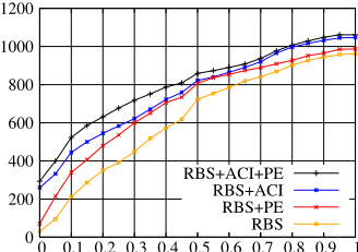
The major motivation behind our +ACI and +PE extensions to RBS is to reduce the size of V RBS required to find a real plan. Figure 1 measures this impact directly.
Both extensions clearly help as intended. Without +ACI, few instances can be solved without search (|V RBS | = 0) as, there, the delete-relaxed plan for the initial state has to be a real plan. The advantage of our extensions remains strong when allowing larger V RBS , until about |V RBS |/|V | = 50% where the gap narrows. After that, the difference is mainly due to benchmarks (like Transport) that ACI solves on the initial state but that are beyond reach of RBS search alone.
7 Conclusion
We have shown that RBS can be synergetically combined with ACI tractable red-black planning, and we have started the exploration of adaptive relaxation refinement within RBS. The results for the former show performance improvements due to the smaller number of black variables that need to be searched over. The results for the latter exhibit promise, but the jury is still out how such adaptive refinement is best done.
Overall, our work contributes another piece in the puzzle how to tap into the power of partial delete relaxation without incurring a prohibitive overhead. This fits into the larger puzzle of how to use informative but costly approximations. We believe that such research is valuable to complement the more prominent focus on fast-but-inaccurate approximations, and we hope that our ideas and insights may be useful for approaches other than red-black planning as well.
Acknowledgments
This work was partially supported by the German Research Foundation (DFG), under grants HO 2169/5-1 ("Critically Constrained Planning via Partial Delete Relaxation") and HO 2169/6-1 ("Star-Topology Decoupled State Space Search").
@inproceedings{ijcai2018p660,
  title     = {Unchaining the Power of Partial Delete Relaxation, Part II: Finding Plans with Red-Black State Space Search},
  author    = {Fickert, Maximilian and Gnad, Daniel and Hoffmann, Joerg},
  booktitle = {Proceedings of the Twenty-Seventh International Joint Conference on
               Artificial Intelligence, {IJCAI-18}},
  publisher = {International Joint Conferences on Artificial Intelligence Organization},
  editor    = {Jérôme Lang},
  pages     = {4750--4756},
  year      = {2018},
  month     = {7},
  note      = {Main track},
  doi       = {10.24963/ijcai.2018/660},
  url       = {https://doi.org/10.24963/ijcai.2018/660},
}
TY - CPAPER TI - Unchaining the Power of Partial Delete Relaxation, Part II: Finding Plans with Red-Black State Space Search AU - Fickert, Maximilian AU - Gnad, Daniel AU - Hoffmann, Joerg T2 - Proceedings of the Twenty-Seventh International Joint Conference on Artificial Intelligence, IJCAI-18 PB - International Joint Conferences on Artificial Intelligence Organization PY - 2018 SP - 4750 EP - 4756 DO - 10.24963/ijcai.2018/660 UR - https://doi.org/10.24963/ijcai.2018/660 ER -Copied
Machine-readable versions of this paper, for tools and AI agents:





