
Analyzing Tie-Breaking Strategies for the A* Algorithm
Proceedings of the Twenty-Seventh International Joint Conference on Artificial Intelligence. Main track. Pages 4715-4721.
https://doi.org/10.24963/ijcai.2018/655
Keywords
- Planning and Scheduling: Theoretical Foundations of Planning
- Planning and Scheduling: Search in Planning and Scheduling
- Heuristic Search and Game Playing: Heuristic Search
Abstract
For a given state space and admissible heuristic function h there is always a tie-breaking strategy for which A* expands the minimum number of states [Dechter and Pearl, 1985]. We say that these strategies have optimal expansion. Although such a strategy always exists it may depend on the instance, and we currently do not know a tie-breaker that always guarantees optimal expansion. In this paper, we study tie-breaking strategies for A*. We analyze common strategies from the literature and prove that they do not have optimal expansion. We propose a novel tie-breaking strategy using cost adaptation that has always optimal expansion. We experimentally analyze the performance of A* using several tie-breaking strategies on domains from the IPC and zero-cost domains. Our best strategy solves significantly more instances than the standard method in the literature and more than the previous state-of-the-art strategy. Our analysis improves the understanding of how to develop effective tie-breaking strategies and our results also improve the state-of-the-art of tie-breaking strategies for A*.
- [Asai and Fukunaga, 2016] Masataro Asai and Alex S Fuku- naga. Tiebreaking strategies for A * search: How to ex- plore the final frontier. In AAAI Conference on Artificial Intelligence, pages 673-679, 2016.
- [Asai and Fukunaga, 2017] Masataro Asai and Alex Fuku- naga. Tie-breaking strategies for cost-optimal best first search. Journal of Artificial Intelligence Research, 58:67- 121, 2017.
- [Dechter and Pearl, 1985] Rina Dechter and Judea Pearl. Generalized best-first search strategies and the optimality of A * . Journal of the ACM, 32(3):505-536, 1985.
- [Hansen and Zhou, 2007] Eric A Hansen and Rong Zhou. Anytime heuristic search. Journal of Artificial Intelligence Research, 28:267-297, 2007.
- [Hart et al., 1968] Peter E. Hart, Nils J. Nilsson, and Bertram Raphael. A formal basis for the heuristic determination of minimum cost paths. IEEE Trans. Systems Science and Cybernetics, 4(2):100-107, 1968.
- [Helmert and Domshlak, 2009] Malte Helmert and Carmel Domshlak. Landmarks, critical paths and abstractions: what's the difference anyway? In International Confer- ence on Automated Planning and Scheduling, pages 162- 169, 2009.
- [Helmert and Röger, 2008] Malte Helmert and Gabriele Röger. How good is almost perfect? In AAAI Confer- ence on Artificial Intelligence, volume 8, pages 944-949, 2008.
- [Helmert, 2006] Malte Helmert. The Fast Downward Plan- ning System. Journal of Artificial Intelligence Research, 26:191-246, 2006.
- [Hoffmann and Nebel, 2001] Jörg Hoffmann and Bernhard Nebel. The FF planning system: Fast plan generation through heuristic search. Journal of Artificial Intelligence Research, 14:253-302, 2001.
- [Holte, 2010] Robert C Holte. Common misconceptions concerning heuristic search. In Symposium on Combina- torial Search, 2010.
- [Richter et al., 2011] Silvia Richter, Matthias Westphal, and Malte Helmert. LAMA 2008 and 2011. In International Planning Competition, pages 117-124, 2011.
References were extracted automatically from the PDF and may contain errors.
Full text extracted automatically from the PDF; figures, tables and equations may differ. The PDF is the version of record.
1 Introduction
A∗ is the most popular best-first heuristic search algorithm [Hart et al., 1968]. It expands states in order of increasing f-values. For a given state s, the function f(s) is the sum of the cost g(s) of the current path from the initial state to state s, and the heuristic cost h(s) from s to a goal state. A heuristic h is admissible if it never overestimates the cost of a state to its closest goal state. In this case A∗ returns an optimal solution path of minimum cost C ∗ , if there is one. The heuristic that returns the cost of an optimal path for all states is called the perfect heuristic h∗ . During the search, it is possible to have several states with the same f-value. Hence, A∗ has to use an order [f, τ] with a tie-breaking strategy τ to select one of them to be expanded next. A∗ with a deterministic tie-breaking strategy τ defines a unique expansion sequence of states.
A state space evaluated by an admissible heuristic h is nonpathological if there exists some cost-optimal path where h(s) < h∗ (s) for all non-goal states s on it. Dechter and Pearl (1985) have shown that in this case the tie-breaker τ plays no role as the set of states with f < C ∗ contains all states expanded by A∗ . However, if the admissible heuristic h on the state space is pathological, then A∗ will expand all states with f < C ∗ and additionally some states with f = C ∗ . This set of states is known as the final plateau or final flayer. There is always a tie-breaking strategy τ that expands, in addition to states with f(s) < C ∗ , only states on a shortest cost-optimal path in the final f-layer (i.e., states along the cost-optimal path with the least number of operators). In this case, we say that tie-breaking strategy τ has optimal expansion, or simply is optimal.
Most of the search and planning literature considers breaking ties in favor of smaller h-values to be a good practice (e.g., [Holte, 2010; Hansen and Zhou, 2007]). Dechter and Pearl (1985) describe A∗ as being agnostic with regard to the tie-breaking strategy letting it "break ties arbitrarily, but in favor of a goal state" and assume that only a few states s will satisfy f(s) = C ∗ . However, Asai and Fukunaga (2016) showed that this is often false and A∗ using tie-breaking strategies that do not favor small h-values can solve more instances and expand fewer states.
In many applications the goal is to minimize the use of some resource (e.g., fuel in logistic problems), and operators that do not use this resource can be modeled as having no cost. Based on this observation Asai and Fukunaga (2016) have introduced so-called zero-cost domains. In such domains, the final plateau can account for a large part of the expanded states and A∗ can follow long zero-cost paths that can be avoided by a tie-breaking strategy.
Empirical analysis shows that all IPC instances using A∗ with heuristic hLM-cut which are solved in 5 minutes or less are pathological and more than 95% of the zero-cost instances solved using this time limit are also pathological. Hence, tiebreakers are relevant for most of the instances in both benchmarks.
In this paper we study tie-breaking strategies for A∗ . We first analyze previously proposed tie-breaking strategies and prove that they are not always optimal. We also propose a new strategy which is guaranteed to have optimal expansion. We experimentally analyze the performance of A∗ using several strategies on the set of IPC instances and instances with zero-cost operators where the perfect heuristic h∗ can be computed. In practical settings using hLM-cut our new strategies solve more instances than other methods in the literature. Our results show how to build an optimal tie-breaking strategy given h∗ and our analysis improves the understanding of how to develop tie-breakers.
2 Background
State Space
Let S = 〈s0, S∗,O, cost〉 be a state space, where s0 is the initial state, S∗ is a set of goal states and O is a set of operators. For a given state s there is a (possibly empty) subset of operators in O that can be applied to s to generate a set of successor states succ(s). Every operator o ∈ O has a cost cost(o) ∈ R+0 associated to a transition s → s′ , where s′ ∈ succ(s). A sequence of distinct states denoted as s0 → s1 → · · · → sn is called a path, if for every pair of consecutive states s → s′ we have s′ ∈ succ(s). If sn ∈ S∗ then the sequence is called a solution path (s-path).
Tie-Breaking Strategies
The A∗ algorithm receives a state space S and a heuristic function h as input and outputs an s-path, if there is one, or "unsolvable" otherwise. A∗ ordering states by [f, τ] with a tie-breaking strategy τ (where f = g + h and τ is some function over S) expands a unique sequence of states 〈s0, s1, . . . , sn〉, called the expansion sequence. We assume that A∗ keeps a priority queue denoted as OPEN that sorts the states lexicographically in increasing order of [f, τ]. To expand a state means to remove it from OPEN and to generate all its successors. Note that in this way goal states are only processed, i.e. removed fromOPEN, but not expanded. If the expansion sequence of A∗ with a given tie-breaking strategy has the minimum number of states among all possible sequences we say that this strategy has optimal expansion - or simply that it is optimal. If the function f uses the perfect heuristic h∗ , we denote it as f ∗ = g + h∗ .
An s-path is not fully informed if h(s) < h∗ (s) for all s /∈ S∗ on that path. Dechter and Pearl (1985) define a state space S with admissible heuristic h to be nonpathological if there exists at least one cost-optimal not fully informed spath. Conversely, a state space S with admissible heuristic h is pathological if all cost-optimal s-paths are fully informed.
3 Common Tie-Breaking Strategies
In this section, we present a theoretical framework to analyze tie-breaking strategies for A∗ . Our framework is based on the perfect heuristic h∗ as a fully informed tie-breaker. In state spaces where we can compute h∗ , A∗ with f ∗ will only expand states whose f-value equals the optimal cost C ∗ . In this setting, the tie-breaking strategy will have optimal expansion if it only expands states on one cost-optimal s-path with the least number of operators.
3.1 Analyzing h∗ as Tie-Breaker
The heuristic search literature usually considers breaking ties by h to be a good approach. Therefore one would expect that when having h∗ , we could use its value as a tie-breaker, leading to an strategy with optimal expansion. In this setting, using order [f ∗ , h∗ ] means that A∗ uses f ∗ as main evaluation function and h∗ as tie-breaker, and any remaining ties are solved arbitrarily.
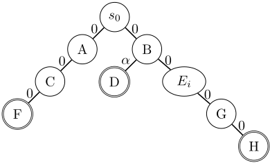
However, using order [f ∗ , h∗ ] is not optimal, as it may expand more states than another strategy. Figure 1a shows an example with two paths to goal states using only zero-cost operators. State s0 is the initial state, doubly-circled states are goals and ellipses represent arbitrarily long transition sequences of zero cost. In this situation, [f ∗ , h∗ ] provides no information. Hence, the expansion sequence depends on how remaining ties are solved, which does not guarantee optimal expansion. To reach a goal from s0, A∗ may expand three states using the left s-path (s0 → A → C → F), or an arbitrarily large set of states using the right s-path (s0 → B → · · · → G → H).
3.2 Analyzing ˆh∗ as Tie-Breaker
Asai and Fukunaga (2017) propose to use distance-to-go heuristics as tie-breakers. A distance-to-go heuristic, denoted ˆh, uses the same algorithm to compute h but replaces the cost of all operators by one. Thus ˆh∗ (s) is the minimum number of operator applications necessary to reach a goal state from s. In practice, A∗ using [f ∗ , ˆh∗ ] improves coverage in zerocost domains [Asai and Fukunaga, 2017].
However, order [f ∗ , ˆh∗ ] can also fail to produce an optimal expansion, as the example of Figure 1a shows. Let α > 0. After expanding s0, we have ˆh∗ (A) = 2, because A can reach the closest goal F applying two operators, and ˆh∗ (B) = 1, because B can reach its closest goal D applying only one operator. As a consequence, A∗ expands state B first. However, the s-path s0 → B → D is not optimal because the operator that enables B to reach goal state F has cost α. Thus [f ∗ , ˆh∗ ] expands four states (〈s0,B,A,C〉), and the optimal strategy only three (〈s0, A, C〉).

4 Novel Strategies based on Cost Adaptation
The tie-breaking strategy using the perfect heuristic h∗ guides the search along a cost-optimal path but fails to identify the cost-optimal path with the least number of operators. The tiebreaking strategy using the distance-to-go heuristic ˆh∗ guides the search along a path with fewest operators to the goal but fails to estimate the total cost of the path. We can combine both estimates to improve the search performance.
Definition 1 (Cost-adapted heuristic). Let S = 〈s0, S∗,O, cost〉 be a state space and h be a heuristic for S. A cost-adapted heuristic hc is a heuristic function for S, where for all o ∈ O there is a new operator oc ∈ Oc with cost(oc) = cost(o) + c and hc computes the heuristic function by replacing O by Oc.
In other words, the cost-adapted heuristic hc is the same algorithm to compute h on S, but adds a constant c to each operator cost. We will call a tie-breaking strategy based on hc a method using cost adaptation.
Richter et al. (2011) introduced the idea of adding one to every operator cost in the satisficing LAMA solver. The intuition is that by doing so, A∗ can combine the operator cost with the cost of applying an operator. In the special case used in the LAMA solver with c = 1 we denote hc as h+1.
4.1 Analyzing h∗c as Tie-Breaking Strategy
Now, we analyze the behavior of h∗c for different magnitudes of c. First, consider c = ϵ where ϵ is a small constant such that ϵ ≪ mino∈O{cost(o) | cost(o) > 0}. The effect of making ϵ very small is that even for the longest path with l operators, the product lϵ is still smaller than the smallest difference between a cost-optimal and a non-cost-optimal s-path. If we apply [f ∗ , h∗ϵ ] to the example of Figure 1a it produces the optimal expansion 〈s0,A,C〉.
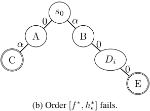
However, [f ∗ , h∗ϵ ] can also fail. Figure 1b shows an example where A∗ with [f ∗ , h∗ϵ ] expands three states and the optimal expansion only two. In this example, after expanding s0, A∗ can expand A and B, where h∗ϵ (A) = α + ϵ while h∗ϵ (B) = 2ϵ + |Di|ϵ. Thus, B is chosen for expansion, followed by the sequence of states Di, leading to goal state E. A∗ expands the path s0 → B → · · · → E instead of the shortest cost-optimal path s0 → A → C.
An approach to solve the example of Figure 1b is to use c = M, where M ≫ maxo∈O(cost(o)). In Figure 1b breaking ties by h∗M produces the optimal expansion. Now, h∗M (A) =
α + M and h∗M (B) = 2M + |Di|M. Since M ≫ α, A∗ expands A instead of B, and terminates at the goal state C, leading the search to the optimal expansion sequence 〈s0, A〉.
However, h∗M fails to achieve the optimal expansion in the example of Figure 1a, where we have h∗M (A) = 2M and h∗M (B) = α + M. Since M ≫ α, we have h∗M (A) > h∗M (B) causing the search to expand B, leading to the same problem of [f ∗ , ˆh∗ ].
Unfortunately, there is no strategy for selecting c that works universally for any task. Figure 2 shows an example where there is no constant c such that order [f ∗ , h∗c ] leads to an optimal expansion. The optimal strategy must expand the path s0 → A → C → X → A′ → C ′ . However, for c > α, after expanding the initial state s0 we have h∗c (B) < h∗c (A) because of the path using the operator with cost α from B to X, and thus A∗ will expand state B which is not optimal. For c < α+ϵ, on the other hand, after expanding state X, A∗ will next select state B′ since h∗c (B′ ) < h∗c (A′ ), but the optimal expansion strategy should expand A′ in order to minimize the number of expansions. Since ϵ > 0 for every c one of the two cases will fail. Despite this, cost adaptation will prove to be useful in defining a tie-breaking strategy with optimal expansion.
5 An Optimal Expansion Strategy with Cost Adaptation
Dechter and Pearl (1985) have shown that for any state space S and admissible heuristic function h there is always a tiebreaking strategy τ such that A∗ with [f, τ] presents optimal expansion. The following theorem presents a strategy using a single tie-breaker that achieves optimal expansion for admissible and consistent heuristic functions h. This expansion strategy only requires the evaluation function f to use a consistent heuristic h - not necessarily h∗ - but it stills need h∗ for the tie-breaker, which now also considers the g values of the states.
Theorem 1. For an admissible and consistent heuristic h, A∗ with order [g + h, τ ] and tie-breaker τ = g + h∗ϵ has optimal expansion.
Proof. If there is no solutionA∗ will always expand all reachable states and thus has optimal expansion. Otherwise, since h is admissible and consistent, A∗ will process states by nondecreasing f-values, ending with f = C ∗ at some goal state. We will show that A∗ with tie-breaker τ expands the least number of states in the final f-layer, from which the claim follows, since states with f < C ∗ must be expanded by all searches which find an optimal solution.
Consider the moment when for the first time the state of least f-value in OPEN has f = C ∗ . From this point on all processed states have f = C ∗ = g + h∗ and therefore are processed in τ -order. For a state s on a cost-optimal path to a goal we have h∗ϵ (s) ≤ h∗ (s) + ϵ ¯ d, where ¯ d is an upper bound on the distance from s to some goal, since a non-cost-optimal path from s to some goal costs at least h∗ (s) +∆ for some ∆ > 0, and therefore h∗ϵ (s) ≤ h∗ (s) + ϵ ¯ d < h∗ + ∆, by choice of ϵ. 1
Thus, for the state s of least τ-value we have τ(s) = g(s) + h∗ϵ (s) = g(s) + h∗ (s) + ϵd∗ (s) where d∗ (s) is the shortest distance from s to a goal on some cost-optimal path, and since g + h∗ is constant for all states with f = C ∗ , they are processed in d∗ -order. Now, since each state of distance d∗ has at least one successor of shortest distance d∗ - 1 on a cost-optimal path, the distance to the goal decreases in each iteration, and A∗ expands exactly d∗ - 1 states before processing a goal state. Since d∗ is the shortest distance on a cost-optimal path, optimal expansion follows.
As a simple consequence of Theorem 1 we have that for A∗ with the perfect heuristic function h∗ , tie-breaker τ = g +h∗ϵ has optimal expansion. Notice that optimal expansion does not imply that A∗ finds a shortest cost-optimal solution, since the shortest path is guaranteed only for the final f-layer.
The result from Theorem 1 is useful from the following perspective: consider an inadmissible heuristic h where h(s) = h∗ (s) in a significant number of states but h(s) > h∗ (s) in only a few. Function h cannot be used to guide an admissible search, but Theorem 1 suggests that we can use it as an effective tie-breaking strategy.
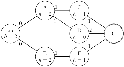
Figure 3 illustrates an instance where order [g + h, g + h∗ϵ ] fails if h is inconsistent. Heuristic values are shown inside each state. To achieve optimal expansion the algorithm should expand paths s0 → A → C → G or s0 → B → E → G. However, whenever we expand state A, we must expand state D as well. Due to the inconsistency of the heuristic function h, we have f(D) < f(A) and argmins∈OPEN f(s) = D, hence this successor must be expanded before than any other successor of A. Since our tie-breaking strategy g + h∗ϵ cannot guarantee to favor the expansion of B over the expansion of A, it does not guarantee optimal expansion if h is inconsistent.
1 For integer costs, we can choose ϵ < 1/ ¯ d.
If instead of using the optimal expansion strategy from Theorem 1, we use [f ∗ , g + hϵ] (i.e., the perfect heuristic is used for the evaluation function and not the tie-breaker), we cannot guarantee optimal expansion anymore. Consider the example of Figure 1a and assume that oα is the operator causing the transition of cost α. Let h be an approximation of h∗ that is incapable of capturing the necessity of applying operator oα - i.e., it considers the cost of operator oα to be 0. Since A∗ uses f ∗ , we have f ∗ (A) = f ∗ (B) = C ∗ = 0 for the successors A and B of s0. To break this tie, we use g + hϵ. We have g + hϵ(A) = 2ϵ and g + hϵ(B) = ϵ due to the possible path s0 → B → D where h cannot predict the need of oα. Hence, B is expanded instead of A, and A∗ fails to expand only the cost-optimal path with the least number of operators.
6 Experiments
In our experiments, we tested the improvement of state expansions, search time and coverage for the different methods studied here and previously mentioned in the literature. The experiments use revision 6251 of the Fast-Downward planning system [Helmert, 2006] with the modifications of Asai and Fukunaga (2017) and also the same benchmarks as them. In total, we used 1104 instances from the IPC and 620 from the zero-cost benchmarks of Asai and Fukunaga (2017). All experiments have been run on a PC with an AMD FX-8150 processor running at 3.6 GHz and 32 GB of main memory. In the case where τ cannot solve all ties, the remaining ones are broken by FIFO order.
6.1 Comparing Theory and Practice
We first focus on the question if the theoretical advantage of cost adaptation strategies translates into practice. For these experiments we use a time limit of 30 minutes, a memory limit of 4GB, and the subset of 183 IPC and 87 zero-cost domains, which could be solved optimally by all methods given these limits and the internal limits of Fast-Downward to build h∗ . Thus, this reduced set of benchmarks contains instances with smaller state spaces than usual.
Table 1 reports the geometric mean of the number of expanded states for different combinations of primary A∗ heuristic and tie-breaker. For each combination, the table shows the results for IPC and zero-cost domains separately. The pair at the header of each column is denoted by h1 , h2 , where h1 was used as the heuristic for the function f and h2 as the heuristic for the tie-breaking strategy. The best results in each column are shown in bold. We can see that using the benchmarks with a small state space, A∗ expands few states.
We first analyze the theoretical predictions using the perfect heuristic h∗ in function f and as tie-breaker. The results are in the first two columns of Table 1. In practice, the theoretically optimal tie-breaker g+h∗ϵ performs best, and strictly dominates the other tie-breakers on zero-cost domains.
In the second combination we relax the tie-breaker to hLM-cut [Helmert and Domshlak, 2009]. As expected, the number of expanded states increases for all tie-breakers, showing that, in fact, tie-breaking strategy matters. The theoretical results do not guarantee an optimal expansion breaking ties by τ = g+h∗ϵ in this case, and indeed we can see that the strategy actually performs worse than other strategies. This can be explained by the fact the hLM-cut is not fully informed. Thus, when a successor state on a cost-optimal path is generated it tends to have a higher value of g + hLM-cut ϵ , and leads A∗ to first expand less informed states. This effect is less pronounced for tie-breakers not using g.
| h∗ , h∗ | h∗ , hLM-cut | hLM-cut , h∗ | hLM-cut , hLM-cut | hLM-cut , hFF | ||||||
|---|---|---|---|---|---|---|---|---|---|---|
| IPC | Z | IPC | Z | IPC | Z | IPC | Z | IPC | Z | |
| [g + h1 , h2 ] | 12.05 | 124.49 | 13.34 | 244.44 | 69.92 | 549.94 | 79.24 | 805.68 | 80.79 | 690.19 |
| [g + h1 , ˆh2 ] | 11.78 | 13.33 | 14.28 | 23.72 | 69.87 | 119.02 | 79.29 | 172.46 | 80.88 | 156.04 |
| [g + h1 , h2+1 ] | 11.78 | 13.37 | 13.01 | 20.18 | 69.87 | 105.57 | 79.18 | 147.79 | 80.95 | 131.62 |
| [g + h1 , h2ϵ ] | 11.78 | 13.39 | 12.63 | 21.33 | 69.88 | 105.57 | 79.36 | 144.93 | 79.63 | 142.02 |
| [g +h1 , g +h2ϵ ] | 11.78 | 13.26 | 31.91 | 65.67 | 69.84 | 104.67 | 80.71 | 145.88 | 81.26 | 141.08 |
In the remaining combinations, we switch roles and focus on not fully informed searches using heuristic hLM-cut with different tie-breakers. In all these cases, A∗ expands a significantly higher number of states. The fifth and sixth column in Table 1 show the results for breaking ties using h∗ . Even though hLM-cut is not guaranteed to be consistent, we find that the f-values never decrease in about 90% of the instances in both benchmarks. Hence, our result from Theorem 1 guarantees optimal expansion for [g + hLM-cut , g + h∗ ] in most instances. In fact, all cost adaptation methods have a similar performance on the IPC instances, and the theoretically optimal tie-breaker g + h∗ϵ is the best method by a small margin.
We finally relax the tie-breaker to approximations of h∗ . Following Asai and Fukunaga (2017) we have selected heuristics hLM-cut and hFF [Hoffmann and Nebel, 2001]. Note that heuristic hFF is not admissible, but will not change the optimality of the search when used as a tie-breaker. Both cases expand more states than the optimal strategy, as expected, but the relative performance of the tie-breakers is very similar, with little difference on the IPC benchmark. On the zero-cost domains, breaking ties by ˆh is always the worst, and methods using cost adaption are always the best.
Table 1 quantifies the advantage of our theoretically best method on the restricted set of small instances, where h∗ can be computed. Yet, some instances still need many expansions when breaking ties using h∗ which is a fully informed heuristic. For example, A∗ with order [g + hLM-cut , h∗ ] or [g+h∗ , h∗ ] expands 349.108 states in the first instance of the ELEVATORS-UP domain, while order [g +hLM-cut , g +h∗ϵ ] expands 18 states. Instance P04 of the same domain presents a similar behavior. In the ROVERS-FUEL domain, instance P05 has an optimal solution of cost C ∗ = 3 with a length of 22 operators, but the order [f ∗ , hLM-cut ] expands 272.171 states, while the order [f ∗ , g + h∗ϵ ] expands exactly 22 states.
In summary, all cost adaptation strategies are similar on the IPC instances, but far better than the default tie-breaker h on zero-cost. Our results show that even in small state spaces and using the perfect heuristic h∗ , tie-breakers are important, even when not optimal. Still, the heuristic function is more important than the tie-breaker, as the comparison between the second and the third combinations confirms. The last two combinations show that tie-breakers also make a difference in practice, and there is enough room for improvement.
| Method | IPC (1104) | Zero-cost (620) |
|---|---|---|
| [f, hLM-cut ] | 525 | 237 |
| [f, ˆhLM-cut ] | 531 | 301 |
| [f, hLM-cut +1 ] | 530 | 299 |
| [f, hLM-cut ϵ ] | 532 | 301 |
| [f, g + hLM-cut ϵ ] | 524 | 300 |
| [f, hFF ] | 548 | 251 |
| [f, ˆhFF ] | 557 | 338 |
| [f, hFF +1 ] | 562 | 352 |
| [f, hFF ϵ ] | 559 | 351 |
| [f, g + hFF ϵ ] | 553 | 346 |
| [f, ˆhFF , 〈d〉 , LIFO] | 530 | 328 |
6.2 Performance on the Complete Set of Instances
We now turn to the practical performance of tie-breakers using cost adaptation. Our second experiment compares the coverage of different tie-breaking strategies using f = g + hLM-cut to guide the search on the complete set of 1104 IPC and 620 zero-cost domains. In this experiment we have imposed limits of 4 GB and 5 min for each run, following Asai and Fukunaga (2017).
The results are shown in Table 2. We compare our main cost adaptation methods against the standard methods in the literature and the current best deterministic tie-breaker on zero-cost domains fromAsai and Fukunaga (2017) (last row). (The best non-deterministic tie-breaker of Asai and Fukunaga (2017) solves in average 2.3 instances more.) Looking at the group of tie-breakers using hLM-cut we find that that all methods using cost adaption perform better than the standard tie-breaker h.
The second group using hFF in the tie-breaker dominates the strategies using hLM-cut only. This confirms the observa-
Number of Expansions
Expansions per Second
tion of Asai and Fukunaga (2017) that breaking ties by hFF is better than hLM-cut . However, we find that ˆhFF also performs better on zero-cost domains than their best strategy. This can probably be explained by the difference between processor speeds. Again the tie-breaker g + hFF ϵ which is theoretically best for h∗ is competitive. The overall best method is hFF +1 . It solves five instances more on the IPC benchmark than ˆhFF , the best tie-breaker from the literature. The best known tiebreaker for zero-cost instances is [f, ˆhFF , 〈d〉 , LIFO] [Asai and Fukunaga, 2017]. Here, hFF +1 solves 24 instances more.
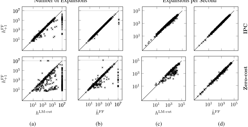
Figures 4a and 4b compare the number of expanded states of the best method [f, hFF +1 ] against the most used method in literature, [f, hLM-cut ] and the best method from the literature [f, ˆhFF ]. The plots on top show results for IPC instances, the ones on the bottom for zero-cost. We see that tie-breaking with hFF +1 expands fewer states on most of the instances compared to hLM-cut , in particular on the zero-cost domains. The number of expanded states compared to ˆhFF is similar in IPC but in zero-cost domains hFF +1 outperforms ˆhFF in general.
Another important issue about tie-breaking strategies is the overhead to compute a second evaluation function. Figures 4c and 4d compare the expansions per second of the methods. We find that all methods expand about the same number of states per second, with the exception of hLM-cut on zero-cost domains.
In general lines, the "pure" cost adaptation methods ([f, hc]) using the hFF heuristic have the best performance. Tie-breaking by hFF +1 presents the best coverage in both benchmarks.
7 Conclusion and FutureWork
In this paper, we presented a tie-breaking strategy for A∗ with h∗ that guarantees the minimum number of expanded states among all tie-breaking strategies. Our analysis showed that even for the perfect heuristic h∗ previously proposed tiebreakers fail in producing an optimal tie-breaking strategy. Our results showed how to build an optimal tie-breaking strategy for A∗ for an admissible and consistent heuristic h.
Our experiments confirm the results from Asai and Fukunaga (2017) that tie-breakers have the potential to increase coverage and reduce the number of expanded states. In summary, our best method based on cost adaptation solves 152 instances more than breaking ties by h, the most common tie-breaker in the literature, and more than the two deterministic methods from Asai and Fukunaga (2017) we have tested. Our experiments showed that even in small state spaces and with the perfect heuristic h∗ , the performance of A∗ can be improved by a better tie-breaking strategy. Our main contribution in this work is to provide an analysis that enables a better understanding of the role of tie-breaking strategies in the performance of A∗ .
Two ideas may be interesting to investigate further. The first is an analysis similar to the one by Helmert and Röger (2008) who investigated for specific domains the performance of A∗ with almost perfect heuristics. One could do the same with almost perfect tie-breakers. Second, one may study the existence of effective domain-dependent tiebreakers, not based on h∗ .
Acknowledgments
This work was supported by FAPERGS as part of project 17/2551 - 0000867.7 and was conducted while the first author was a student at the Federal University of Rio Grande do Sul.
@inproceedings{ijcai2018p655,
  title     = {Analyzing Tie-Breaking Strategies for the A* Algorithm},
  author    = {Corrêa, Augusto B. and Pereira, André G. and Ritt, Marcus},
  booktitle = {Proceedings of the Twenty-Seventh International Joint Conference on
               Artificial Intelligence, {IJCAI-18}},
  publisher = {International Joint Conferences on Artificial Intelligence Organization},
  editor    = {Jérôme Lang},
  pages     = {4715--4721},
  year      = {2018},
  month     = {7},
  note      = {Main track},
  doi       = {10.24963/ijcai.2018/655},
  url       = {https://doi.org/10.24963/ijcai.2018/655},
}
TY - CPAPER TI - Analyzing Tie-Breaking Strategies for the A* Algorithm AU - Corrêa, Augusto B. AU - Pereira, André G. AU - Ritt, Marcus T2 - Proceedings of the Twenty-Seventh International Joint Conference on Artificial Intelligence, IJCAI-18 PB - International Joint Conferences on Artificial Intelligence Organization PY - 2018 SP - 4715 EP - 4721 DO - 10.24963/ijcai.2018/655 UR - https://doi.org/10.24963/ijcai.2018/655 ER -Copied
Machine-readable versions of this paper, for tools and AI agents:





