
Think Globally, Embed Locally --- Locally Linear Meta-embedding of Words
Proceedings of the Twenty-Seventh International Joint Conference on Artificial Intelligence. Main track. Pages 3970-3976.
https://doi.org/10.24963/ijcai.2018/552
Keywords
- Natural Language Processing: Natural Language Semantics
- Machine Learning: Deep Learning
- Machine Learning Applications: Applications of Unsupervised Learning
- Natural Language Processing: Natural Language Processing
Abstract
Distributed word embeddings have shown superior performances in numerous Natural Language Processing (NLP) tasks.
However, their performances vary significantly across different tasks,
implying that the word embeddings learnt by those methods capture complementary aspects of lexical semantics.
Therefore, we believe that it is important to combine the existing word embeddings to produce more accurate and complete
meta-embeddings of words.
For this purpose, we propose an unsupervised locally linear meta-embedding learning method that takes
pre-trained word embeddings as the input, and produces more accurate meta embeddings.
Unlike previously proposed meta-embedding learning methods that learn a global projection over all words in a vocabulary,
our proposed method is sensitive to the differences in local neighbourhoods of the individual source word embeddings.
Moreover, we show that vector concatenation, a previously proposed highly competitive baseline
approach for integrating word embeddings, can be derived as a special case of the proposed method.
Experimental results on semantic similarity, word analogy, relation classification, and short-text classification tasks show that our
meta-embeddings to significantly outperform prior methods in several benchmark datasets,
establishing a new state of the art for meta-embeddings.
- [Bansal et al., 2014] Mohit Bansal, Kevin Gimpel, and Karen Livescu. Tailoring continouos word representations for dependency parsing. In Proc. of ACL, 2014.
- [Bruni et al., 2012] Elia Bruni, Gemma Boleda, Marco Ba- roni, and Nam Khanh Tran. Distributional semantics in technicolor. In Proc. of ACL, pages 136-145, 2012.
- [Chen et al., 2013] Yanqing Chen, Bryan Perozzi, Rami Al- Rfou, and Steven Skiena. The expressive power of word embeddings. In Proc. of ICML Workshop, 2013.
- [Collobert and Weston, 2008] Ronan Collobert and Jason Weston. A unified architecture for natural language pro- cessing: Deep neural networks with multitask learning. In Proc. of ICML, pages 160 -167, 2008.
- [Firth, 1957] John R. Firth. A synopsis of linguistic theory 1930-55. Studies in Linguistic Analysis, pages 1 -32, 1957.
- [Goikoetxea et al., 2016] Josu Goikoetxea, Eneko Agirre, and Aitor Soroa. Single or multiple? combining word rep- resentations independently learned from text and wordnet. In Proc. of AAAI, pages 2608-2614, 2016.
- [Hill et al., 2014] Felix Hill, Kyunghyun Cho, Sébastian Jean, Coline Devin, and Yoshua Bengio. Not all neural embeddings are born equal. In NIPS workshop, 2014.
- [Hill et al., 2015a] Felix Hill, Kyunghyun Cho, Sébastian Jean, Coline Devin, and Yoshua Bengio. Embedding word similarity with neural machine translation. In ICLR Work- shop, 2015.
- [Hill et al., 2015b] Felix Hill, Roi Reichart, and Anna Ko- rhonen. Simlex-999: Evaluating semantic models with (genuine) similarity estimation. Computational Linguis- tics, 41(4):665-695, 2015.
- [Huang et al., 2012] Eric H. Huang, Richard Socher, Christopher D. Manning, and Andrew Y. Ng. Improving word representations via global context and multiple word prototypes. In Proc. of ACL, pages 873-882, 2012.
- [Jurgens et al., 2012] David A. Jurgens, Saif Mohammad, Peter D. Turney, and Keith J. Holyoak. Measuring degrees of relational similarity. In Proc. of SemEval, 2012.
- [Kibriya and Frank, 2007] Ashraf M. Kibriya and Eibe Frank. An empirical comparison of exact nearest neigh- bout algorithms. In Proc. of PKDD, pages 140-151, 2007.
- [Luo et al., 2014] Yong Luo, Jian Tang, Jun Yan, Chao Xu, and Zheng Chen. Pre-trained multi-view word embedding using two-side neural network. In Proc. of AAAI, pages 1982-1988, 2014.
- [Luong et al., 2013] Minh-Thang Luong, Richard Socher, and Christopher D. Manning. Better word representations with recursive neural networks for morphology. In CoNLL, 2013.
- [Mikolov et al., 2013a] Tomas Mikolov, Kai Chen, and Jef- frey Dean. Efficient estimation of word representation in vector space. In Proc. of ICLR, 2013. [Mikolov et al., 2013b] Tomas Mikolov, Ilya Sutskever, Kai Chen, Gregory S. Corrado, and Jeffrey Dean. Distributed representations of words and phrases and their composi- tionality. In Proc. of NIPS, pages 3111-3119, 2013.
- [Miller and Charles, 1998] G. Miller and W. Charles. Con- textual correlates of semantic similarity. Language and Cognitive Processes, 6(1):1-28, 1998.
- [Mnih and Hinton, 2009] Andriy Mnih and Geoffrey E. Hin- ton. A scalable hierarchical distributed language model. In D. Koller, D. Schuurmans, Y. Bengio, and L. Bottou, editors, Proc. of NIPS, pages 1081-1088. 2009.
- [Pennington et al., 2014] Jeffery Pennington, Richard Socher, and Christopher D. Manning. Glove: global vectors for word representation. In Proc. of EMNLP, pages 1532-1543, 2014.
- [Rubenstein and Goodenough, 1965] H. Rubenstein and J.B. Goodenough. Contextual correlates of synonymy. Com- munications of the ACM, 8:627-633, 1965.
- [Saul and Roweis, 2003] Lawrence K. Saul and Sam T. Roweis. Think globally, fit locally: Unsupervised learn- ing of low dimensional manifolds. Journal of Machine Learning Research, 4:119-115, 2003.
- [Socher et al., 2013] Richard Socher, Alex Perelygin, Jean Wu, Jason Chuang, Christopher D. Manning, Andrew Ng, and Christopher Potts. Recursive deep models for seman- tic compositionality over a sentiment treebank. In Proc. of EMNLP, pages 1631-1642, 2013.
- [Tian et al., 2016] Yingtao Tian, Vivek Kullkarni, Bryan Per- ozzi, and Steven Skiena. On the convergent properties of word embedding methods. arXiv, 2016.
- [Tsuboi, 2014] Yuta Tsuboi. Neural networks leverage corpus-wide information for part-of-speech tagging. In Proc. of EMNLP, pages 938-950, 2014.
- [Turian et al., 2010] Joseph Turian, Lev Ratinov, and Yoshua Bengio. Word representations: A simple and general method for semi-supervised learning. In Proc. of ACL, pages 384 -394, 2010.
- [Turney and Pantel, 2010] Peter D. Turney and Patrick Pan- tel. From frequency to meaning: Vector space models of semantics. Journal of Aritificial Intelligence Research, 37:141 -188, 2010.
- [Vylomova et al., 2016] Ekaterina Vylomova, Laura Rimell, Trevor Cohn, and Timothy Baldwin. Take and took, gaggle and goose, book and read: Evaluating the utility of vector differences for lexical relational learning. In ACL, pages 1671-1682, 2016.
- [Yin and Schütze, 2016] Wenpeng Yin and Hinrich Schütze. Learning meta-embeddings by using ensembles of embed- ding sets. In Proc. of ACL, pages 1351-1360, 2016.
- [Zou et al., 2013] Will Y. Zou, Richard Socher, Daniel Cer, and Christopher D. Manning. Bilingual word embeddings for phrase-based machine translation. In Proc. of EMNLP, pages 1393-1398, 2013.
References were extracted automatically from the PDF and may contain errors.
Full text extracted automatically from the PDF; figures, tables and equations may differ. The PDF is the version of record.
1 Introduction
Representing the meanings of words is a fundamental task in Natural Language Processing (NLP). A popular approach to represent the meaning of a word is to embed it in some fixed-dimensional vector space [Turney and Pantel, 2010]. In contrast to sparse and high-dimensional counting-based distributional word representation methods that use co-occurring contexts of a word as its representation, dense and lowdimensional prediction-based distributed word representations [Pennington et al., 2014; Mikolov et al., 2013a; Huang et al., 2012; Collobert and Weston, 2008; Mnih and Hinton, 2009] have obtained impressive performances in numerous NLP tasks such as sentiment classification [Socher et al., 2013], and machine translation [Zou et al., 2013].
Previous works studying the differences in word embedding learning methods [Chen et al., 2013; Yin and Sch¨utze, 2016] have shown that word embeddings learnt using different methods and from different resources have significant variation in quality and characteristics of the semantics captured. For example, [Hill et al., 2014; Hill et al., 2015a] showed that the word embeddings trained from monolingual vs. bilingual corpora capture different local neighbourhoods. Bansal et al. [2014] showed that an ensemble of different word representations improves the accuracy of dependency parsing, implying the complementarity of the different word embeddings. This suggests the importance of metaembedding - creating a new embedding by combining different existing embeddings. We refer to the input word embeddings to the meta-embedding process as the source embeddings. Yin and Sch¨utze [2016] showed that by metaembedding five different pre-trained word embeddings, we can overcome the out-of-vocabulary problem, and improve the accuracy of cross-domain part-of-speech (POS) tagging. Encouraged by the above-mentioned prior results, we expect an ensemble containing multiple word embeddings to produce better performances than the constituent individual embeddings in NLP tasks.
There are three main challenges a meta-embedding learning method must overcome.
First, the vocabularies covered by the source embeddings might be different because they have been trained on different text corpora. Therefore, not all words will be equally represented by all of the source embeddings. Even in situations where the implementations of the word embedding learning methods are publicly available, it might not be possible to retrain those embeddings because the text corpora on which those methods were originally trained might not be publicly available. Moreover, it is desirable if the meta-embedding method does not require the original resources upon which they were trained such as corpora or lexicons, and can directly work with the pre-trained word embeddings. This is particularly attractive from a computational point of view because re-training source embedding methods on large corpora might require significant processing times and resources.
Second, the vector spaces and their dimensionalities of the source embeddings might be different. In most predictionbased word embedding learning methods the word vectors are randomly initialised. Therefore, there is no obvious correspondence between the dimensions in two word embeddings learnt even from two different runs of the same method, let alone from different methods [Tian et al., 2016]. Moreover, the pre-trained word embeddings might have different dimensionalities, which is often a hyperparameter determined experimentally. This becomes a challenging task when incorporating multiple source embeddings to learn a single metaembedding because the alignment between the dimensionalities of the source embeddings is unknown.
Third, the local neighbourhoods of a particular word under different word embeddings show a significant diversity. For example, as the nearest neighbours of the word bank, GloVe [Pennington et al., 2014], a word sense insensitive embedding, lists credit, financial, cash, whereas word sense sensitive embeddings created by Huang et al. [2012] lists river, valley, marsh when trained on the same corpus. We see that the nearest neighbours for the different senses of the word bank (i.e. financial institution vs. river bank) are captured by the different word embeddings. Meta-embedding learning methods that learn a single global projection over the entire vocabulary are insensitive to such local variations in the neighbourhoods [Yin and Sch¨utze, 2016].
To overcome the above-mentioned challenges, we propose a locally-linear [Saul and Roweis, 2003] meta-embedding learning method that (a) requires only the words in the vocabulary of each source embedding, without having to predict embeddings for missing words, (b) can meta-embed source embeddings with different dimensionalities, (c) is sensitive to the diversity of the neighbourhoods of the source embeddings.
Our proposed method comprises of two steps: a neighbourhood reconstruction step (Section 3.2), and a projection step (Section 3.3). Meta-embedding learning can be seen as a mutlivariate regression problem of mapping source word embeddings to a common meta-embedding space. In the simplest case of linear regression, this requires learning a transformation in the order of source vocabulary size times meta embedding vocabulary size, which leads to data sparseness issues. However, as suggested by the distributional hypothesis [Firth, 1957], the meaning of a word is mostly influenced by its local neighbours. Therefore, as the first step, we represent the embedding of a word by the linearly weighted combination of the embeddings of its nearest neighbours in each source embedding space. This is equivalent to assuming that the weight matrix of regression is sparse, and it greatly reduces the number of parameters. The weights we learn are shared across different source embeddings, thereby incorporating the information from different source embeddings in the meta-embedding. Interestingly, vector concatenation, which has found to be an accurate meta-embedding method, can be derived as a special case of this reconstruction step.
Next, the projection step computes the meta-embedding of each word such that the nearest neighbours in the source embedding spaces are embedded closely to each other in the meta-embedding space. The reconstruction weights can be efficiently computed using stochastic gradient descent, whereas the projection can be efficiently computed using a truncated eigensolver.
It is noteworthy that we do not directly compare different source embeddings for the same word in the reconstruction step nor in the projection step. This is important because the dimensions in source word embeddings learnt using different word embedding learning methods are not aligned. Moreover, a particular word might not be represented by all source embeddings. This property of the proposed method is attractive because it obviates the need to align source embeddings, or predict missing source word embeddings prior to metaembedding. Therefore, all three challenges described above are solved by the proposed method.
The above-mentioned properties of the proposed method enables us to compute meta-embeddings for five different source embeddings covering 2.7 million unique words. We evaluate the meta-embeddings learnt by the proposed method on semantic similarity prediction, analogy detection, relation classification, and short-text classification tasks. The proposed method significantly outperforms several competitive baselines and previously proposed meta-embedding learning methods [Yin and Sch¨utze, 2016] on multiple benchmark datasets.
2 RelatedWork
Yin and Sch¨utze [2016] proposed a meta-embedding learning method (1TON) that projects a meta-embedding of a word into the source embeddings using separate projection matrices. The projection matrices are learnt by minimising the sum of squared Euclidean distance between the projected source embeddings and the corresponding original source embeddings for all the words in the vocabulary. They propose an extension (1TON+) to their meta-embedding learning method that first predicts the source word embeddings for out-ofvocabulary words in a particular source embedding, using the known word embeddings. Next, 1TON method is applied to learn the meta-embeddings for the union of the vocabularies covered by all of the source embeddings.
Experimental results in semantic similarity prediction, word analogy detection, and cross-domain POS tagging tasks show the effectiveness of both 1TON and 1TON+. In contrast to our proposed method, which learns locally-linear projections that are sensitive to the variations in the local neighbourhoods in the source embeddings, 1TON and 1TON+ can be seen as globally linear projections between meta and source embedding spaces. As we see later in Section 4.4, our proposed method outperforms both of those methods consistently in all benchmark tasks demonstrating the importance of neighbourhood information when learning meta-embeddings. Moreover, our proposed meta-embedding method does not directly compare different source embeddings, thereby obviating the need to predict source embeddings for out-of-vocabulary words. Locally-linear embeddings [Saul and Roweis, 2003] are attractive from a computational point-of-view as well because during optimisation we require information from only the local neighbourhood of each word.
Although not learning any meta-embeddings, several prior work have shown that by incorporating multiple word embeddings learnt using different methods improve performance in various NLP tasks. For example, Tsuboi [2014] showed that by using both word2vec and GloVe embeddings together in a POS tagging task, it is possible to improve the tagging accuracy, if we had used only one of those embeddings. Similarly, Turian et al. [2010] collectively used Brown clusters, CW and HLBL embeddings, to improve the performance of named entity recognition and chucking tasks.
Luo et al. [2014] proposed a multi-view word embedding learning method that uses a two-sided neural network. They adapt pre-trained CBOW [Mikolov et al., 2013b] embeddings from Wikipedia and click-through data from a search engine. Their problem setting is different from ours because their source embeddings are trained using the same word embedding learning method but on different resources whereas, we consider source embeddings trained using different word embedding learning methods and resources. Although their method could be potentially extended to meta-embed different source embeddings, the unavailability of their implementation prevented us from exploring this possibility.
Goikoetxea et al. [2016] showed that concatenation of word embeddings learnt separately from a corpus and the WordNet to produce superior word embeddings. Moreover, performing Principal Component Analysis (PCA) on the concatenated embeddings slightly improved the performance on word similarity tasks. In Section 4.3, we discuss the relationship between the proposed method and vector concatenation.
3 Locally Linear Meta-Embeddings
3.1 Problem Settings
To explain the proposed meta-embedding learning method, let us consider two source word embeddings, denoted by S1 and S2. Although we limit our discussion here to two source embeddings for the simplicity of the description, the proposed meta-embedding learning method extends the locally linear embedding method originally proposed by Saul and Roweis [2003] such that it can be applied to any number of source embeddings.
We denote the dimensionalities of S1 and S2 respectively by d1 and d2 (in general, d1 ̸= d2). The sets of words covered by each source embedding (i.e. vocabulary) are denoted by V1 and V2. The source embedding of a word v ∈ V1 is represented by a vector v(1) ∈ Rd1 , whereas the same for a word v ∈ V2 by a vector v(2) ∈ Rd2 . Let the set union of V1 and V2 be V = {v1, . . . , vn} containing n words. In particular, note that our proposed method does not require a word v to be represented by all source embeddings, and can operate on the union of the vocabularies of the source embeddings. The meta-embedding learning problem is then to learn an embedding v(P) ∈ RdP in a meta-embedding space P with dimensionality dP for each word v ∈ V.
3.2 Nearest Neighbour Reconstruction
We reconstruct each word v ∈ V separately from its knearest neighbours N1(v), and N2(v), respectively in S1 and S2. The reconstruction weight wvu assigned to a neighbour u ∈ N1(v) ∪ N2(v) is found by minimising the reconstruction error Φ(W) defined by (1), which is the sum of local distortions in the two source embedding spaces.
Words that are not k-nearest neighbours of v in either of the source embedding spaces will have their weights set to zero (i.e. wvu = 0, ∀u /∈ N1(v) ∪ N2(v)). Moreover, we require the sum of reconstruction weights for each v to be equal to one (i.e. ∑u∈V wuv = 1).
To compute the weights wvu that minimise (1), we compute its error gradient ∂Φ(W) ∂wvu as follows:
Here, the indicator function, I[x], returns 1 if x is true and 0 otherwise. We uniformly randomly initialise the weights wvu for each neighbour u of v, and use stochastic gradient descent (SGD) with the learning rate scheduled by AdaGrad to compute the optimal values of the weights. The initial learning rate is set to 0.01 and the maximum number of iterations to 100 in our experiments. Empirically we found that these settings to be adequate for convergence. Finally, we normalise the weights wuv for each v such that they sum to 1 (i.e. ∑u∈V wvu = 1).
Exact computation of k nearest neighbours for a given data point in a set of n points requires all pairwise similarity computations. Because we must repeat this process for each data point in the set, this operation would require a time complexity of O(n3 ). This is prohibitively large for the vocabularies we consider in NLP where typically n > 103 . Therefore, we resort to approximate methods for computing k nearest neighbours. Specifically, we use the BallTree algorithm [Kibriya and Frank, 2007] to efficiently compute the approximate k-nearest neighbours, for which the time complexity of tree construction is O(n log n) for n data points.
The solution to the least square problem given by (1), subjected to the summation constraints, can be found by solving a set of linear equations. Time complexity of this step is O(N(d1|N1|3 + d2|N2|3 )), which is cubic in the neighbourhood size and linear in both the dimensionalities of the embeddings and vocabulary size. However, we found that the iterative estimation process using SGD described above to be more efficient in practice. Because k is significantly smaller than the number of words in the vocabulary, and often the word being reconstructed is contained in the neighbourhood, the reconstruction weight computation converges after a small number (less than 5 in our experiments) of iterations.
3.3 Projection toMeta-Embedding Space
In the second step of the proposed method, we compute the meta-embeddings v(P) ,u(P) ∈ RdP for words v, u ∈ V using the reconstruction weights wvu we computed in Section 3.2. Specifically, the meta-embeddings must minimise the projection cost, Ψ(P), defined by (2).
By finding a P space that minimises (2), we hope to preserve the rich neighbourhood diversity in all source embeddings within the meta-embedding. The two summations in (2) over N1(v) and N2(v) can be combined to re-write (2) as follows:
Here, w′uv is computed using (4).
The dP dimensional meta-embeddings are given by the eigenvectors corresponding to the smallest (dP + 1) eigenvectors of the matrix M given by (5).
Here, W′ is a matrix with the (v, u) element set to w′vu . The smallest eigenvalue of M is zero and the corresponding eigenvector is discarded from the projection. The eigenvectors corresponding to the next smallest dP eigenvalues of the symmetric matrix M can be found without performing a full matrix diagonalisation.Operations involving M such as the left multiplication by M, which is required by most sparse eigensolvers, can exploit the fact that M is expressed in (5) as the product between two sparse matrices. Moreover, truncated randomised methods can be used to find the smallest eigenvectors, without performing full eigen decompositions. In our experiments, we set the neighbourhood sizes for all words in all source embeddings equal to n (i.e ∀i |Ni(v)| = N, ∀v ∈ V), and project to a dP(<N) dimensional meta-embedding space. Source code for our implementation is available. 1
4 Experiments and Results
4.1 SourceWord Embeddings
We use five previously proposed pre-trained word embedding sets as the source embeddings in our experiments:
HLBL: (hierarchical log-bilinear) [Mnih and Hinton, 2009] embeddings released by Turian et al. [2010] (246,122 word embeddings, 100 dimensions, trained on Reuters Newswire (RCV1) corpus).
Huang: Huang et al. [2012] used global contexts to train multi-prototype word embeddings that are sensitive to word senses (100,232 word embeddings, 50 dimensions, trained on April 2010 snapshot of Wikipedia).
GloVe: Pennington et al. [2014] used global co-occurrences of words over a corpus to learn word embeddings (1,193,514 word embeddings, 300 dimensions, trained on 42 billion corpus of web crawled texts).
CW: Collobert and Weston [2008] learnt word embeddings following a multitask learning approach covering multiple NLP tasks (we used the version released by Turian et al. [2010] trained on the same corpus as HLBL containing 268,810 word embeddings, 200 dimensions).
1 https://github.com/LivNLP/LLE-MetaEmbed
CBOW: Mikolov et al. [2013b] proposed the continuous bag-of-words method to train word embeddings (we discarded phrase embeddings and selected 929,922 word embeddings, 300 dimensions, trained on the Google News corpus containing ca. 100 billion words).
The intersection of the five vocabularies is 35,965 words, whereas their union is 2,788,636. Although any word embedding can be used as a source we select the above-mentioned word embeddings because (a) our goal in this paper is not to compare the differences in performance of the source embeddings, and (b) by using the same source embeddings as in prior work [Yin and Sch¨utze, 2016], we can perform a fair evaluation. 2 In particular, we could use word embeddings trained by the same algorithm but on different resources, or different algorithms on the same resources as the source embeddings. We defer such evaluations to an extended version of this conference submission.
4.2 Evaluation Tasks
We evaluate the meta-embeddings using four extrinsic tasks: Semantic similarity measurement: We measure the similarity between two words as the cosine similarity between the corresponding embeddings, and measure the Spearman correlation coefficient against the human similarity ratings. We use Rubenstein and Goodenough's dataset [Rubenstein and Goodenough, 1965] (RG) rare words dataset (RW) [Luong et al., 2013], Stanford's contextual word similarities (SCWS) [Huang et al., 2012], the MEN dataset [Bruni et al., 2012], and the SimLex dataset [Hill et al., 2015b] (SL). In addition, we use the Miller and Charles' dataset [Miller and Charles, 1998] (MC) as a validation dataset to tune various hyperparameters such as the neighbourhood size, and the dimensionality of the meta-embeddings for the proposed method and baselines.
Word analogy detection: Using the CosAdd method, we solve word-analogy questions in the Google dataset (GL) [Mikolov et al., 2013b], and in the SemEval (SE) dataset [Jurgens et al., 2012]. Specifically, for three given words a, b and c, we find a fourth word d that correctly answers the question a to b is c to what? such that the cosine similarity between the two vectors (b-a+c) and d is maximised.
Relation classification: We use the DiffVec (DV) [Vylomova et al., 2016] dataset containing 12,458 triples of the form (relation, word1, word2) covering 15 relation types. We train a 1-nearest neighbour classifier where for each target tuple we measure the cosine similarity between the vector offset for its two word embeddings, and those of the remaining tuples in the dataset. If the top ranked tuple has the same relation as the target tuple, then it is considered to be a correct match. We compute the (micro-averaged) classification accuracy over the entire dataset as the evaluation measure.
Short-text classification: We use two binary short-text classification datasets: Stanford sentiment treebank (TR) 3 and the movie reviews dataset (MR) 4 . Each review is represented as a bag-of-words and we compute the centroid of the embeddings of the words in each bag to represent that review. Next, we train a binary logistic regression classifier with a cross-validated ℓ2 regulariser using the train portion of each dataset, and evaluate the classification accuracy using the test portion of the dataset.
2 Although skip-gram embeddings are shown to outperform most other embeddings, they were not used as a source by Yin and Sch¨utze [2016]. Therefore, to be consistent in comparisons against prior work, we decided not to include skip-gram as a source.
4.3 Baselines
Concatenation (CONC): A simple but an accurate baseline for creating meta-embeddings is to concatenate all source embeddings [Yin and Sch¨utze, 2016]. Each source embedding is ℓ2 normalised prior to concatenation such that they contribute equally to similarity computations. 5
Interestingly, CONC can be seen as a special case in the reconstruction step described in Section 3.2. To see this, let us denote the concatenation of column vectors v(1) and v(2) by x = (v(1) ; v(2) ), and u(1) and u(2) by y = (u(1) ;u(2) ), where x, y ∈ Rd1+d2 . Then, the reconstruction error defined by (1) can be written as follows:
The common neighbourhood N(v) in (6) can be obtained by either limiting N(v) to N1(v) ∩ N2(v) or, by extending the neighbourhoods to the entire vocabulary (N(v) = V). (6) shows that under those neighbourhood constraints, the first step in our proposed method can be seen as reconstructing the neighbourhood of the concatenated space. The second step would then find metaembeddings that preserve the locally linear structure in the concatenated space. One drawback of concatenation is that it increases the dimensionality of the metaembeddings compared to the source-embeddings, which might be problematic when storing or processing the meta-embeddings. For example, for the five source embeddings we use here dP = 100+50+300+200+300 = 950.
Singular Value Decomposition (SVD): We create an N × 950 matrix C by arranging the CONC vectors for the union of all source embedding vocabularies. For words that are missing in a particular source embedding, we assign zero vectors of that source embedding's dimensionality. Next, we perform SVD on C = UDV⊤, where U and V are unitary matrices and the diagonal matrix D contains the singular values of C. We then select the d largest left singular vectors from U to create a dP dimensional embeddings for the N words. Using the MC validation dataset, we set dP = 300. 6
3 http://nlp.stanford.edu/sentiment/treebank.html
4 http://www.cs.cornell.edu/people/pabo/movie-review-data/
5 As reported by [Yin and Sch¨utze, 2016], we found that CONC performs poorly without emphasising GloVe and CBOW by a constant factor, which is set to 8 using MC as a validation dataset.
6 Multiplying U by the singular values, a technique used to weight
4.4 Meta-Embedding Results
Using the MC dataset, we find the best values for the neighbourhood size n = 1200 and dimensionality dP = 300 for the Proposed method. Experimental results for different methods on different tasks/datasets are shown in Table 1, where rows 1-5 show the performance of the individual source embeddings. Next, we perform ablation tests (rows 6-20), where we hold-out one source embedding at a time. We evaluate statistical significance against best performing individual source embedding on each dataset. For the semantic similarity benchmarks we use Fisher transformation to compute p<0.05 confidence intervals for Spearman correlation coefficients. In all other (classification) datasets, we used Clopper-Pearson binomial exact confidence intervals at p<0.05.
Among the individual source embeddings, we see that GloVe and CBOW stand out as the two best source embeddings, which is further confirmed by the ablation results. Performing SVD (rows 11-15) after concatenating, does not always result in an improvement. SVD is a global projection that reduces the dimensionality of the meta-embeddings created via concatenation. This result indicates that different source embeddings might require different levels of dimensionality reductions, and applying a single global projection does not always guarantee improvements. Ensemble methods that use all five source embeddings are shown in rows 21-25. 1TON and 1TON+ are proposed by Yin and Sch¨utze [2016], and were detailed in Section 2. Because they did not evaluate on all tasks that we do here, to conduct a fair and consistent evaluation we used their publicly available metaembeddings 7 without retraining by ourselves.
Overall, from Table 1, we see that the Proposed method (row 25) obtains the best performance in all tasks/datasets. In 6 out of 12 benchmarks, this improvement is statistically significant over the best single source embedding. Moreover, in the MEN dataset (the largest among the semantic similarity benchmarks compared in Table 1 with 3000 word-pairs), and the Google dataset, the improvements of the Proposed method over the previously proposed 1TON and 1TON+ are statistically significant.
The ablation results for the Proposed method show that, overall, by using all source embeddings we can obtain the best results. Different source embeddings are trained from different resources and by optimising different objectives. Therefore, for different words, the local neighbours predicted by different source embeddings will be complementary. Unlike the other methods, the Proposed method never compares different source embeddings' vectors directly, but only via the neighbourhood reconstruction weights. Consequently, the Proposed method is unaffected by relative weighting of source embeddings. In contrast, the CONC is highly sensitive against the weighting. In fact, we confirmed that the performance scores of the CONC method were decreased by 3-10 points when we did not do the weight tuning described in Section 4.2. The unnecessity of the weight tuning is thus a clear advantage of the Proposed method.
the latent dimensions, did not result in any notable improvements in our experiments.
7 http://cistern.cis.lmu.de/meta-emb/
| Model | RG | MC | WS | RW | SCWSMEN | SL | GL | SE | DV | SA | MR | ||
|---|---|---|---|---|---|---|---|---|---|---|---|---|---|
| 1 | GloVe | 81.7 | 80.8 | 64.3 | 38.4 | 54.0 | 74.3 | 37.4 | 70.5 | 39.9 | 87.7 | 73.4 | 70.0 |
| 2 | CBOW | 76.0 | 82.2 | 69.8 | 53.4 | 53.4 | 78.2 | 44.2 | 75.2 | 39.1 | 87.4 | 73.6 | 71.0 |
| sources 3 | HLBL | 35.3 | 49.3 | 35.7 | 19.1 | 47.7 | 30.7 | 22.1 | 16.6 | 34.8 | 72.0 | 62.6 | 61.6 |
| 4 | Huang | 51.3 | 58.8 | 58.0 | 36.4 | 63.7 | 56.1 | 21.7 | 8.3 | 35.2 | 76.0 | 64.8 | 60.9 |
| 5 | CW | 29.9 | 34.3 | 28.4 | 15.3 | 39.8 | 25.7 | 15.6 | 4.7 | 34.6 | 75.6 | 62.7 | 61.4 |
| 6 | CONC (-GloVe) | 75.0 | 79.0 | 70.0 | 55.3 | 62.9 | 77.7 | 41.5 | 64.0 | 38.7 | 82.9 | 72.1 | 69.1 |
| 7 | CONC (-CBOW) | 80.8 | 81.0 | 65.2 | 46.0 | 56.3 | 74.9 | 37.3 | 70.0 | 38.8 | 86.0 | 71.6 | 69.9 |
| 8 | CONC (-HLBL) | 83.0 | 84.0 | 71.9 | 53.4 | 61.4 | 80.1∗ | 41.6 | 72.7 | 39.5 | 84.9 | 71.0 | 69.4 |
| 9 | CONC (-Huang) | 83.0 | 84.0 | 71.6 | 48.8 | 60.8 | 80.1∗ | 41.9 | 72.8 | 40.0 | 86.7 | 71.2 | 69.1 |
| 10 | CONC (-CW) | 82.9 | 84.0 | 71.9 | 53.3 | 61.6 | 80.2∗ | 41.6 | 72.6 | 39.6 | 84.9 | 72.3 | 69.9 |
| 11 | SVD (-GloVe) | 78.6 | 79.9 | 68.4 | 53.9 | 61.6 | 77.5 | 40.1 | 61.7 | 38.5 | 84.1 | 71.6 | 69.8 |
| 12 | SVD (-CBOW) | 80.5 | 81.2 | 64.4 | 45.3 | 55.3 | 74.2 | 35.7 | 70.9 | 38.7 | 86.7 | 73.4 | 69.1 |
| ablation 13 | SVD (-HLBL) | 82.7 | 83.6 | 70.3 | 52.6 | 60.1 | 79.9∗ | 39.6 | 73.5 | 39.8 | 87.3 | 73.2 | 70.4 |
| 14 | SVD (-Huang) | 82.5 | 85.0 | 70.3 | 48.6 | 59.8 | 79.9∗ | 39.9 | 73.7 | 40.0 | 87.3 | 73.5 | 70.8 |
| 15 | SVD (-CW) | 82.5 | 83.9 | 70.4 | 52.5 | 60.1 | 80.0∗ | 39.7 | 73.3 | 39.8 | 87.2 | 73.1 | 70.7 |
| 16 | Proposed (-GloVe) | 79.8 | 79.7 | 71.1 | 54.7 | 62.3 | 78.2 | 46.1 | 84.2∗ | 39.8 | 85.4 | 72.2 | 70.2 |
| 17 | Proposed (-CBOW) | 80.9 | 82.1 | 67.4 | 58.7∗ | 58.7 | 75.7 | 45.2 | 85.2∗ | 40.1 | 87.1 | 73.8 | 70.1 |
| 18 | Proposed (-HLBL) | 82.1 | 86.1 | 71.3 | 58.3∗ | 62.1 | 81.9∗ | 34.8 | 86.3∗ | 40.3 | 87.7 | 73.7 | 71.1 |
| 19 | Proposed (-Huang) | 81.2 | 85.2 | 73.1 | 55.1 | 63.7 | 81.4∗ | 42.3 | 82.6∗ | 41.1 | 87.5 | 73.9 | 71.2 |
| 20 | Proposed (-CW) | 83.1 | 84.8 | 72.5 | 58.5 | 62.3 | 81.1∗ | 43.5 | 88.4∗ | 41.9 | 87.8 | 71.6 | 71.1 |
| 21 | CONC | 82.9 | 84.1 | 71.9 | 53.3 | 61.5 | 80.2∗ | 41.6 | 72.9 | 39.6 | 84.9 | 72.4 | 69.9 |
| 22 | SVD | 82.7 | 83.9 | 70.4 | 52.6 | 60.0 | 79.9∗ | 39.7 | 73.4 | 39.7 | 87.2 | 73.4 | 70.7 |
| ensemble 23 | 1TON | 80.7 | 80.7 | 74.5 | 60.1∗ | 61.6 | 73.5 | 46.4 | 76.8 | 42.3∗ | 87.6 | 73.8 | 70.3 |
| 24 | 1TON+ | 82.7 | 85.0 | 75.3 | 61.6∗ | 60.2 | 74.1 | 46.3 | 77.0 | 40.1 | 83.9 | 73.9 | 69.2 |
| 25 | Proposed | 83.4 | 86.2 | 75.7∗ | 62.8∗ | 63.8 | 82.2∗ | 48.7 | 89.9∗ | 43.1∗ | 88.7∗ | 74.0 | 71.3 |
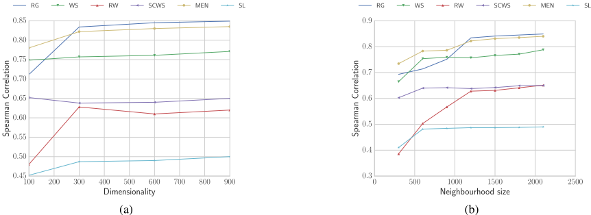
To investigate the effect of the dimensionality dP on the meta-embeddings learnt by the proposed method, in Figure 1a, we fix the neighbourhood size N = 1200 and measure the performance on semantic similarity measurement tasks when varying dP . Overall, we see that the performance peaks around dP = 300. Such behaviour can be explained by the fact that smaller dP dimensions are unable to preserve information contained in the source embeddings, whereas increasing dP beyond the rank of the weight matrix W is likely to generate noisy eigenvectors.
In Figure 1b, we study the effect of increasing the neighbourhood size n equally for all words in all source embeddings, while fixing the dimensionality of the meta-embedding dP = 300. Initially, performance increases with the neighbourhood size and then saturates. This implies that in practice a small local neighbourhood is adequate to capture the differences in source embeddings.
5 Conclusion
We proposed an unsupervised locally linear method for learning meta-embeddings from a set of source embeddings. Experiments on several NLP tasks show the accuracy of the proposed method, which outperforms previously proposed meta-embedding learning methods on multiple benchmark datasets. In future, we plan to extend the proposed method to learn cross-lingual meta-embeddings.
@inproceedings{ijcai2018p552,
  title     = {Think Globally, Embed Locally --- Locally Linear Meta-embedding of Words},
  author    = {Bollegala, Danushka and Hayashi, Kohei and Kawarabayashi, Ken-ichi},
  booktitle = {Proceedings of the Twenty-Seventh International Joint Conference on
               Artificial Intelligence, {IJCAI-18}},
  publisher = {International Joint Conferences on Artificial Intelligence Organization},
  editor    = {Jérôme Lang},
  pages     = {3970--3976},
  year      = {2018},
  month     = {7},
  note      = {Main track},
  doi       = {10.24963/ijcai.2018/552},
  url       = {https://doi.org/10.24963/ijcai.2018/552},
}
TY - CPAPER TI - Think Globally, Embed Locally --- Locally Linear Meta-embedding of Words AU - Bollegala, Danushka AU - Hayashi, Kohei AU - Kawarabayashi, Ken-ichi T2 - Proceedings of the Twenty-Seventh International Joint Conference on Artificial Intelligence, IJCAI-18 PB - International Joint Conferences on Artificial Intelligence Organization PY - 2018 SP - 3970 EP - 3976 DO - 10.24963/ijcai.2018/552 UR - https://doi.org/10.24963/ijcai.2018/552 ER -Copied
Machine-readable versions of this paper, for tools and AI agents:





