
A Generic Approach for Accelerating Stochastic Zeroth-Order Convex Optimization
Proceedings of the Twenty-Seventh International Joint Conference on Artificial Intelligence. Main track. Pages 3040-3046.
https://doi.org/10.24963/ijcai.2018/422
Keywords
- Machine Learning: Machine Learning
- Uncertainty in AI: Uncertainty in AI
Abstract
In this paper, we propose a generic approach for accelerating the convergence of existing algorithms to solve the problem of stochastic zeroth-order convex optimization (SZCO). Standard techniques for accelerating the convergence of stochastic zeroth-order algorithms are by exploring multiple functional evaluations (e.g., two-point evaluations), or by exploiting global conditions of the problem (e.g., smoothness and strong convexity). Nevertheless, these classic acceleration techniques are necessarily restricting the applicability of newly developed algorithms. The key of our proposed generic approach is to explore a local growth condition (or called local error bound condition) of the objective function in SZCO. The benefits of the proposed acceleration technique are: (i) it is applicable to both settings with one-point evaluation and two-point evaluations; (ii) it does not necessarily require strong convexity or smoothness condition of the objective function; (iii) it yields an improvement on convergence for a broad family of problems. Empirical studies in various settings demonstrate the effectiveness of the proposed acceleration approach.
- [Agarwal et al., 2010] Alekh Agarwal, Ofer Dekel, and Lin Xiao. Optimal algorithms for online convex optimization with multi-point bandit feedback. In COLT, pages 28-40, 2010.
- [Bolte et al., 2015] Jérôme Bolte, Trong Phong Nguyen, Juan Peypouquet, and Bruce Suter. From error bounds to the complexity of first-order descent methods for convex functions. CoRR, abs/1510.08234, 2015.
- [Chen et al., 2011] Po-Lung Chen, Chen-Tse Tsai, Yao-Nan Chen, Ku-Chun Chou, Chun-Liang Li, Cheng-Hao Tsai, Kuan-Wei Wu, Yu-Cheng Chou, Chung-Yi Li, Wei-Shih Lin, et al. A linear ensemble of individual and blended models for music rating prediction. In KDD-Cup, pages 21-60, 2011.
- [Dani et al., 2008] Varsha Dani, Sham M Kakade, and Thomas P Hayes. The price of bandit information for on- line optimization. In NIPS, pages 345-352, 2008.
- [Duchi et al., 2015] John C Duchi, Michael I Jordan, Mar- tin J Wainwright, and Andre Wibisono. Optimal rates for zero-order convex optimization: The power of two func- tion evaluations. IEEE Transactions on Information Theo- ry, 61(5):2788-2806, 2015.
- [Flaxman et al., 2005] Abraham D Flaxman, Adam Tauman Kalai, and H Brendan McMahan. Online convex optimiza- tion in the bandit setting: gradient descent without a gra- dient. In SODA, pages 385-394, 2005.
- [Hazan and Kale, 2014] Elad Hazan and Satyen Kale. Be- yond the regret minimization barrier: optimal algorithm- s for stochastic strongly-convex optimization. Journal of Machine Learning Research, 15(1):2489-2512, 2014.
- [Lian et al., 2016] Xiangru Lian, Huan Zhang, Cho-Jui H- sieh, Yijun Huang, and Ji Liu. A comprehensive linear speedup analysis for asynchronous stochastic parallel op- timization from zeroth-order to first-order. In NIPS, pages 3054-3062, 2016.
- [Nakamura et al., 2017] Nathan Nakamura, Jason Seepaul, Joseph B Kadane, and B Reeja-Jayan. Design for low- temperature microwave-assisted crystallization of ceramic thin films. Applied Stochastic Models in Business and In- dustry, 2017. [Nemirovski et al., 2009] Arkadi Nemirovski, Anatoli Judit- sky, Guanghui Lan, and Alexander Shapiro. Robust s- tochastic approximation approach to stochastic program- ming. SIAM Journal on Optimization, 19(4):1574-1609, 2009.
- [Nesterov and Spokoiny, 2017] Yurii Nesterov and Vladimir Spokoiny. Random gradient-free minimization of convex functions. Foundations of Computational Mathematics, 17(2):527-566, 2017.
- [Shamir, 2013] Ohad Shamir. On the complexity of ban- dit and derivative-free stochastic convex optimization. In COLT, pages 3-24, 2013.
- [Shamir, 2017] Ohad Shamir. An optimal algorithm for bandit and zero-order convex optimization with two- point feedback. Journal of Machine Learning Research, 18(52):1-11, 2017.
- [Sokolov et al., 2016] Artem Sokolov, Julia Kreutzer, Stefan Riezler, and Christopher Lo. Stochastic structured predic- tion under bandit feedback. In NIPS, pages 1489-1497, 2016.
- [Wang et al., 2017] Yining Wang, Simon Du, Sivaraman Balakrishnan, and Aarti Singh. Stochastic zeroth-order optimization in high dimensions. arXiv preprint arX- iv:1710.10551, 2017.
- [Wibisono et al., 2012] Andre Wibisono, Martin J Wain- wright, Michael I Jordan, and John C Duchi. Finite sam- ple convergence rates of zero-order stochastic optimiza- tion methods. In NIPS, pages 1439-1447, 2012.
- [Xu et al., 2016] Yi Xu, Qihang Lin, and Tianbao Yang. Ac- celerated stochastic subgradient methods under local error bound condition. arXiv preprint arXiv:1607.01027, 2016.
- [Xu et al., 2017] Yi Xu, Qihang Lin, and Tianbao Yang. S- tochastic convex optimization: Faster local growth implies faster global convergence. In ICML, pages 3821-3830, 2017.
- [Yang and Lin, 2015] Tianbao Yang and Qihang Lin. Rs- g: Beating subgradient method without smoothness and strong convexity. arXiv preprint arXiv:1512.03107, 2015.
- [Zadorozhnyi et al., 2016] Oleksandr Zadorozhnyi, Gun- thard Benecke, Stephan Mandt, Tobias Scheffer, and Mar- ius Kloft. Huber-norm regularization for linear prediction models. In ECML, pages 714-730, 2016.
- [Zinkevich, 2003] Martin Zinkevich. Online convex pro- gramming and generalized infinitesimal gradient ascent. In ICML, pages 928-936, 2003.
References were extracted automatically from the PDF and may contain errors.
Full text extracted automatically from the PDF; figures, tables and equations may differ. The PDF is the version of record.
1 Introduction
We consider the following problem of stochastic convex optimization:
where Ω ⊆ Rd is a closed compact convex set, f(x; ξ) is a stochastic convex function depending on random noise ξ. This problem has broad applications in computer science and engineering. For example, many practical problems in machine learning can be cast into a stochastic convex optimization, where ξ denotes a random data point and x denotes the parameter of a prediction model. A standard approach for solving the problem of Eq. (1) is to adopt the stochastic (sub)gradient of f(x; ξ) [Nemirovski et al., 2009]. However, there exist situations where the first-order gradient information is computationally infeasible, expensive, or impossible, while the zeroth-order functional information can be easily obtained. For example, in online auctions and advertisement selections, only function values are revealed as feedbacks for algorithms [Wibisono et al., 2012]. In stochastic structured predictions, explicit differentiations may be difficult to perform while the functional evaluations of predicted structures are easily obtained [Sokolov et al., 2016]. The optimization problem of Eq. (1) in such situations is referred to SZCO.
A key concern in the development of iterative stochastic zeroth-oder algorithms for solving Eq. (1) is the order of the necessary number of functional evaluations in the form of f(x; ξ), which is termed as sample complexity or iteration complexity. [Flaxman et al., 2005] should be the first work related to SZCO. They studied a closely related setting namely online bandit convex optimization where only one-point evaluation (OPE) is available for the cost function at each iteration. Applied to the stochastic setting, their algorithm suffers from an iteration complexity of O(d2 /ϵ4 ) for finding an ϵ-optimal solution ̂x such that E[f(̂x) -minx∈Ω f(x)] ≤ ϵ. Since then, there have been a number of studies [Agarwal et al., 2010; Shamir, 2013; Duchi et al., 2015; Shamir, 2017; Nesterov and Spokoiny, 2017] trying to improve the iteration complexity of [Flaxman et al., 2005] in online bandit setting or in stochastic optimization setting. A useful technique to accelerate the convergence of SZCO is by leveraging twopoint evaluations (TPE) at each iteration. Another technique is to explore the strong convexity or the smoothness condition of the random function f(x; ξ). Clearly, both techniques impose strong restrictions of their developed algorithms, and thus the applicability of the resultant algorithms is limited.
1.1 Our Contributions
The goal of this paper is to design a generic approach for accelerating existing SZCO algorithms which is applicable to both settings with OPE and TPE, and to cases even without smoothness and strong convexity assumptions of the objective function. A novel contribution is to explore a generic local growth condition (or called local error bound condition) of the objective function, which specifies how fast the objective function grows in a local neighborhood of optimal solutions. In particular, we propose a generic algorithmic framework for accelerating existing SZCO algorithms in various settings by leveraging the local error bound condition. This is accomplished by a novel synthesis of existing SZCO algorithms and a multi-stage adaptive technique, which consists of three components: using a multi-stage scheme with each stage running existing algorithms, warm starting each stage using the solution from previous stage, and adaptively changing the algorithm's parameters after each stage (e.g., step size, the smoothing parameter). Depending on the local error bound (LEB) condition, the improvement over existing results is up to a factor of 1/ϵ2 . Empirical studies in various settings demonstrate the effectiveness of the proposed acceleration approach.
1.2 RelatedWork
A quick comparison between our obtained upper bounds of iteration complexities under different settings and previous upper bounds is shown in Table 1. Lower bounds for SZCO have been also studied in several works [Dani et al., 2008; Shamir, 2013; Duchi et al., 2015] in different settings. We will show that our proposed algorithm's performance in certain settings matches the existing lower bounds. For example, for stochastic zeroth-order linear optimization with OPE, our obtained upper bound of iteration complexity is ˜O(d2 /ϵ2 )1 , which matches the lower bound in [Dani et al., 2008]. In addition, the best upper bound in this paper for SZCO in the setting with OPE without smoothness assumption is ˜O(d2 /ϵ2 ), which matches the lower bound in [Shamir, 2013] up to a logarithmic factor. It is also notable that the best upper bound achieved in this paper can be as good as min(O(d2 log(1/ϵ)), ˜O(d/ϵ)). However, we note that our result does not contradict to the lower bound in [Duchi et al., 2015] because either their considered random functions do not necessarily have bounded gradients as assumed in this paper or their considered problem does not satisfy the LEB condition that yields our best result. Finally, we note that the LEB condition has been explored in (stochastic) convex optimization for improving the convergence of first-order methods [Yang and Lin, 2015; Xu et al., 2017]. To the best of our knowledge, this is the first paper that leverages the LEB condition for improving the convergence of SZCO.
2 Notations and Preliminaries
In this section, we present some notations and preliminaries for SZCO. Let the ℓ-norm of a vector x be ‖x‖ℓ (where ℓ ≥ 1). The inner product of two vectors x, y is denoted by x⊤y = 〈x, y〉. The notation of B(x, r) denotes a Euclidean ball centered at x with radius r > 0. The ceiling integer of a real number r is ⌈r⌉.
1 We omit a poly-logarithmic factor for ˜O(·).
Let ∂f(x) and ∇f(x) denote, respectively, the subgradient of a non-smooth function and the gradient of a smooth function. f(x) is G-Lipschitz continuous if ∃G > 0 such that |f(x) - f(y)| ≤ G‖x - y‖2, ∀x, y ∈ Ω, i.e., ‖∂f(x)‖2 ≤ G, ∀x ∈ Ω. f(x) is L-smooth if it is differentiable and has L-Lipschitz-continuous gradient, i.e., ‖∇f(x) - ∇f(y)‖2 ≤ L‖x - y‖2, ∀x, y ∈ Ω. f(x) is convex if f(x) ≥ f(y)+〈∂f(y), x-y〉, ∀x, y ∈ Ω. f(x) is σ-strongly convex if f(x) ≥ f(y)+〈∂f(y), x-y〉+σ‖xy‖22 /2, ∀x, y ∈ Ω and σ ≥ 0.
Let u ∼ B(0, 1) denote a noise vector uniformly sampled from a unit sphere, and u ∼ N(0, 1) denote a noise vector sampled from a standard Gaussian distribution. Given a noise vector u, let ˆ f(x; ξ) ≜ Eu[f(x + δu; ξ)] denote a smoothed function with smoothing parameter δ > 0 and ˆ f(x) ≜ Eu;ξ[f(x + δu; ξ)]. Let Ω∗ denote the optimal solution set for Eq. (1), and f∗ ≜ minx∈Ω f(x). In the sequel, we will make the following assumption.
Assumption 1. Assume that there exist x0 ∈ Ω and ϵ0 > 0 such that f(x0) -minx∈Ω f(x) ≤ ϵ0. For any δ ∈ (0, +∞), there exists B > 0 such that |f(x + δu; ξ)| ≤ B for any x ∈ Ω and ξ, where u ∼ B(0, 1).
2.1 Noisy Gradient Estimators
The noisy gradient estimator in the setting with OPE proposed by [Flaxman et al., 2005] is given as:
where ut ∼ B(0, 1) and δ > 0. The properties of gft and ˆ f(x; ξ) are stated below.
Lemma 1 ([Flaxman et al., 2005]). Given u ∼ B(0, 1), we have Eu[gft ] = ∇ ˆ f(xt; ξt), and ‖gft ‖2 ≤ dB/δ. If f(x; ξ) is G-Lipschitz continuous, we have |f(x; ξ) - ˆ f(x; ξ)| ≤ Gδ. If f(x; ξ) is L-smooth, we have |f(x; ξ)- ˆ f(x; ξ)| ≤ Lδ2 /2.
For the setting with TPE, there are different gradient estimators used in previous studies. For example, [Agarwal et al., 2010; Shamir, 2017] used the following noisy gradient estimator with ut ∼ B(0, 1):
[Nesterov and Spokoiny, 2017; Duchi et al., 2015] considered the following noisy gradient estimator for TPE with ut ∼ N (0, 1):
The properties of estimators in Eqs. (3) and (4) are summarized as below.
Lemma 2 ([Agarwal et al., 2010; Shamir, 2017]). Given u ∼ B(0, 1), we have Eu[ga t ] = ∇ˆ f(xt; ξt). If f(x; ξ) is G-Lipschitz continuous, we have ‖ga t ‖2 ≤ Gd, Eu[‖ga t ‖22 ] ≤ db2G2C, and |f(x; ξ)- ˆ f(x; ξ)| ≤ Gδ, where C is a universal constant and b is a constant such that (E[‖u‖42 ])1/4 ≤ b. If f(x; ξ) is L-smooth, we have |f(x; ξ)- ˆ f(x; ξ)| ≤ Lδ2 /2.
| setting | algorithm | assumption | iteration complexity | high probability or expectation |
|---|---|---|---|---|
| [Flaxman et al., 2005] | LC | O ( d2 ϵ4 ) | expectation | |
| [Agarwal et al., 2010] | LC + SC LC + SC + SM | ˜O ( d2 ϵ3 ) ˜O ( d2 ϵ2 ) | expectation expectation | |
| OPE | our work | LC + LEB | ˜O ( d2 ϵ2(2-θ) ), θ ∈ (0, 12 ] ˜O ( d2 ϵ2(2-θ) ), θ ∈ (0, 1] | expectation high probability |
| our work | LC + LEB + SM | ˜O ( d2 ϵ3-2θ ), θ ∈ (0, 12 ] ˜O ( d2 ϵ3-2θ ), θ ∈ (0, 1] | expectation high probability | |
| [Agarwal et al., 2010] | LC LC + SC | O ( d2 ϵ2 ) ˜O ( d2 ϵ ) | high probability high probability | |
| [Nesterov and Spokoiny, 2017] | LC LC + SM | ˜O ( d2 ϵ2 ) O ( d ϵ2 ) | expectation expectation | |
| TPE | [Duchi et al., 2015] | LC LC + SM | ˜O ( d log d ϵ2 ) O ( d ϵ2 ) | expectation expectation |
| [Shamir, 2017] | LC | O ( d ϵ2 ) | expectation | |
| our work | LC + LEB | ˜O ( d2 ϵ2(1-θ) ), θ ∈ (0, 1] | high probability | |
| our work | LC + LEB | ˜O ( d ϵ2(1-θ) ), θ ∈ (0, 12 ] | expectation |
Lemma 3 ([Nesterov and Spokoiny, 2017]). Considering u ∼ N(0, 1), we have Eu[gn t ] = ∇ˆ f(xt; ξt). If f(x; ξ) is G-Lipschitz continuous, we have Eu[‖gn t ‖22 ] ≤ G2 (d + 4)2 , and |f(x; ξt)- ˆ f(x; ξt)| ≤ δGd1/2 . If f(x; ξ) is G-Lipschitz continuous and L-smooth, we have Eu[‖gn t ‖22 ] ≤ δ2 (d + 6)3L2 /2 + 2(d + 4)G2 , and |f(x; ξ) - ˆ f(x; ξ)| ≤ δ2Ld/2.
Remark 1: The absolute upper bound of the noisy gradient estimators is needed for high probability analysis and the variance bound of the noisy gradient estimators is useful for expectational convergence analysis.
The iterative update in the previous studies takes the following form:
where η > 0 is a step size, gt is a gradient estimator and ΠΩ denotes the Euclidean projection onto the set Ω. We synthesize the convergence analysis of stochastic optimization in the following proposition, which, combined with properties of different gradient estimators, yields corresponding convergence results in previous studies.
Proposition 1. Considering the update in Eq. (5) with an initial point of x1 ∈ Ω, for any x ∈ Ω, we have
2.2 Local Error Bound (LEB) Condition
Definition 1. A problem of Eq. (1) satisfies the LEB condition on a compact set Ω if there exist θ ∈ (0, 1] and c > 0 such that for any x ∈ Ω
where dist(x, Ω∗) ≜ minv∈Ω∗ ‖v - x‖2.
Note that the LEB condition has been studied thoroughly in [Yang and Lin, 2015; Bolte et al., 2015; Xu et al., 2017]. It is satisfied for a broad family of problems. For example, when f(x) is continuous and semi-algebraic (or subanalytic), the LEB condition holds on any compact set [Bolte et al., 2015]. Below, we consider several instances of problems that satisfy the LEB condition. More interesting examples in machine learning can be found in [Yang and Lin, 2015; Xu et al., 2017].
Algorithm 1 A generic approach for accelerating SZCO
- 1: initialization x0, K, η1, δ1, D1
- 2: for k = 1, · · · ,K do
- 3: x1k = xk-1, Dk = Ω∩B(x1k ,Dk)
- 4: for τ = 1, · · · , t do
- 5: compute a gradient estimator in light of Eq. (2) or Eq. (3) or Eq. (4)
- 6: compute xτk according to Eq. (5) or Eq. (7) with a step size ηk, a parameter δk, and a domain Dk
- 7: end for
- 8: let xk = ∑tτ=1 xτk /t
- 9: update δk+1, Dk+1 and ηk+1
- 10: end for
- 11: return xK
Example 1: When f(x; ξ) = x⊤ξ is a linear function and Ω is a polyhedral set (e.g., hypercube), then the problem of Eq. (1) satisfies the LEB with θ = 1 [Yang and Lin, 2015]. These functions are considered in online bandit linear optimization [Dani et al., 2008]. More generally, if f(x) is a polyhedral function and Ω is a polyhedral set, then LEB with θ = 1 holds [Yang and Lin, 2015]. For instance, f(x) = ∑ni=1 |a⊤i x - bi|/n and Ω = {‖x‖1 ≤ s}.
Example 2: When f(x) is strongly convex, then the LEB condition holds with θ = 1/2 [Xu et al., 2017].
Example 3: Even when f(x) is not strongly convex, the LEB condition with θ = 1/2 may still hold, such as f(x) = ∑ni=1 (a⊤i x - bi)2 /n and Ω is a polyhedral set.
3 Our Generic Approach
In this section, we propose a generic algorithm for accelerating the convergence of SZCO and its main results in various settings. In order to achieve improved high probability convergence results, we need to use the following update to control the last term in Proposition 1:
where D = Ω ∩ B(x1 ,D) with x1 being a reference point and D being the radius of the ball. The proposed acceleration framework is presented in Algorithm 1, which is a multi-stage adaptive scheme consisting of three key components: (i) a multi-stage scheme with each stage running existing updates, (ii) warm starting each stage using the solution from previous stage, and (iii) adaptively changing the parameters after each stage. Next, we present the iteration complexities of Algorithm 1 in various settings. Let ϵk = ϵ0/2k be a sequence.
Theorem 1 (Results for OPE). Let Algorithm 1 run with Eq. (2) as the noisy gradient estimator and K = ⌈log2(ϵ0/ϵ)⌉ stages. We have the following results.
- R-I: if f(x; ξ) is G-Lipschitz continuous, by employing Eq. (5) and setting t = O(d2 /ϵ2(2-θ) ), δk = ϵk/(6G), ηk = ϵ3k /(54G2d2B2 ), then Algorithm 1 enjoys an iteration complexity of ˜O(d2 /ϵ2(2-θ) ) in expectation for problems satisfy the LEB condition with θ ∈ (0, 1/2];
- R-II: if f(x; ξ) is G-Lipschitz continuous and L-smooth, by employing Eq. (5) and setting t = O(d2 /ϵ3-2θ ),
- δk = √ϵk/(√3L), ηk = 2ϵ2k /(9Ld2B2 ), then Algorithm 1 enjoys an iteration complexity of ˜O(d2 /ϵ3-2θ ) in expectation for problems satisfy the LEB condition with θ ∈ (0, 1/2];
- R-III: if f(x; ξ) is G-Lipschitz continuous, by employing Eq. (7) and setting δk, ηk similarly as in R-I and t = ˜O(d2 /ϵ2(2-θ) ),Dk = O(ϵθk-1 ), then Algorithm 1 enjoys an iteration complexity of ˜O(d2 /ϵ2(2-θ) ) with high probability 1-p, where we set p ∈ (0, 1), for problems satisfy the LEB condition with θ ∈ (0, 1];
- R-IV: if f(x; ξ) is G-Lipschitz continuous and L-smooth, by employing Eq. (7) and setting δk, ηk similarly as in R-II and t = ˜O(d2 /ϵ3-2θ ),Dk = O(ϵθk-1 ), then Algorithm 1 enjoys an iteration complexity of ˜O(d2 /ϵ3-2θ ) with high probability 1 - p, where we set p ∈ (0, 1), for problems satisfy the LEB condition with θ ∈ (0, 1].
Remark 2: For the statement of high probability results, we omit a poly-logarithmic factor of log(K/p) in t. Our iteration complexities by leveraging the LEB condition are better than those in [Agarwal et al., 2010; Flaxman et al., 2005]. For LEB with θ = 1/2 that is weaker than the strong convexity assumption, our iteration complexities match that in [Agarwal et al., 2010] for strongly convex functions. For problems with f(x; ξ) being a linear function and Ω being a polyhedral set, the LEB with θ = 1 holds and we achieve an iteration complexity of ˜O(d2 /ϵ2 ) with high probability, which matches the lower bound in [Dani et al., 2008]. Besides, one may get expectational results for θ > 1/2 from high probability results R-III and R-IV following the Corollary 3 in [Xu et al., 2016].
Theorem 2 (Results for TPE). Let Algorithm 1 run with K = ⌈log2(ϵ0/ϵ)⌉ stages. We have the following results.
- R-I: if f(x; ξ) is G-Lipschitz continuous, by employing the noisy gradient estimator of Eq. (3) and the update of Eq. (5) and setting t = O(d/ϵ2(1-θ) ), δk = ϵk/(6G), ηk = 2ϵk/(3db2G2C) where b and C are parameters discussed in Lemma 2, then Algorithm 1 enjoys an iteration complexity of ˜O(d/ϵ2(1-θ) ) in expectation for problems satisfy the LEB condition with θ ∈ (0, 1/2];
- R-II: if f(x; ξ) is G-Lipschitz continuous and L-smooth, by employing the noisy gradient estimator of Eq. (4) and the update of Eq. (5) and setting t = O(d/ϵ2(1-θ) ), δk = √ϵk/(2√dL), ηk = min{ϵk/(4(d + 4)G2 ), 2d/((d + 6)3L)}, then Algorithm 1 enjoys an iteration complexity of ˜O(d/ϵ2(1-θ) ) in expectation for problems satisfy the LEB condition with θ ∈ (0, 1/2];
- R-III: if f(x; ξ) is G-Lipschitz continuous, by employing the noisy gradient estimator of Eq. (3) and the update of Eq. (7) and setting δk = ϵk/(8G), ηk = ϵk/(2d2G2 ), t = ˜O(d2 /ϵ2(1-θ) ), and Dk = O(ϵθk-1 ), then Algorithm 1 enjoys an iteration complexity of ˜O(d2 /ϵ2(1-θ) ) with high probability 1 - p, where we set p ∈ (0, 1), for problems satisfy the LEB condition with θ ∈ (0, 1].
Remark 3: It is notable that in the setting with TPE, the smoothness of the random function does not improve the convergence (by comparing R-I and R-II). The reason is that, for R-I, we utilize the refined analysis in [Shamir, 2017] to bound the variance of the noisy gradient estimator E[‖ga t ‖22 ] ≤ O(d) (see Lemma 2), which is in the same order to that of the noisy gradient estimator gn t with small enough δ as established in [Nesterov and Spokoiny, 2017] (see Lemma 3). The expectational results R-I and R-II have better dependence on d compared to the high probability result R-III. The reason is that, for high probability analysis, we have to use the absolute bound of ga t . However, the expectational results R-I and R-II cannot enjoy better dependence on ϵ for θ > 1/2 as in the high probability result R-III. We notice that one can obtain similar expectational results for θ > 1/2 in light of R-III with the same technique in Remark 2.
Finally, we would like to point out that although the above results require knowing the value of θ in the LEB condition, we can use another level of restarting on top of Algorithm 1 and an increasing sequence of t for the outer loop similar to that in [Yang and Lin, 2015; Xu et al., 2017], which still enjoy improved iteration complexities compared with previous results. Due to limitation of space, this result and the related proofs are both omitted here.
Convergence Analyses. Due to limitation of space, we present proofs of results R-I and R-III in Theorem 1. However, we note that proofs of other results can be simply derived by using different variance bounds of the noisy gradient estimators and different bounds of |f(x; ξ) - ˆ f(x; ξ)| from Lemmas 1-3.
Proof of R-I. Based on Proposition 1 and Lemma 1, we have
By setting ˆxT = ∑Tt=1 xt/T and taking the expectation over randomness in u and ξ, we have
By adopting the generic framework in Algorithm 1, for the k-th stage, we have
where we use t iterations in inner loops of Algorithm 1.
We will prove by induction that E[f(xk) - f∗] ≤ ϵk. It is trivial for k = 0 due to Assumption 1. Conditioned on the inequality of E[f(xk-1) - f∗] ≤ ϵk-1, we will show that E[f(xk) - f∗] ≤ ϵk. Let xk-1,∗ = argminv∈Ω∗ ‖v -
where the second inequality uses the concavity of (s)2θ for θ ≤ 1/2 and the Jensen's inequality. To establish E[f(xk) - f∗] ≤ ϵk, we set
By setting ϵK = ϵ0/2K = ϵ, we have K = ⌈log(ϵ0/ϵ)⌉. Thus, we have E[f(xK) - f∗] ≤ ϵK ≤ ϵ. As a result, the total iteration complexity is ˜O(d2 /ϵ2(2-θ) ).
Proof of R-III. First, ∑Tt=1 ( ˆ f(xt) - ˆ f(x)) ≤ ∑Tt=1 〈gft , (xt -x)〉+∑Tt=1 (∇ ˆ f(xt)-gft )⊤(xt-x). We can use the result in Proposition 1 and the absolute upper bound of the noisy gradient estimator to bound the first term in R.H.S. The second term can be bounded using martingale inequalities (please refer to Lemma 14 in [Hazan and Kale, 2014]). As a result, for any fixed x ∈ Ω ∩ B(x1,D) and ˜ p ∈ (0, 1), with a probability at least 1-˜ p, the following inequality holds
where we use Dk = cϵθk-1 , and xk-1,∗ ∈ B(xk-1,Dk). We can easily establish f(xk) - f∗ ≤ ϵk with high probability by induction if we set δk = O(ϵk), ηk = O(ϵ3k /d2 ), t = O(d2 log(1/˜ p)/ϵ2(2-θ) ). Then, with K = ⌈log(ϵ0/ϵ)⌉, we have the iteration complexity as ˜O(d2 /ϵ2(2-θ) ) with probability of 1 - p, where ˜ p = p/K.
4 Experiments
In this section, we conduct experiments on two real-world datasets in various settings to demonstrate the superior performance of the proposed acceleration approach in Algorithm 1. We run experiments in a personal computer with Intel CPU@3.70GHz and 16GB memory.
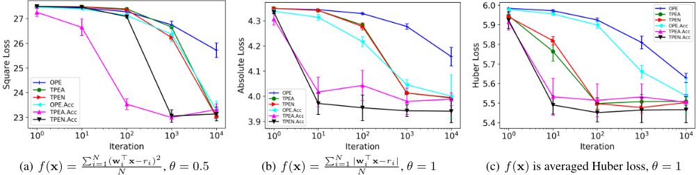
To compare the efficiency of the acceleration framework with prior methods, we will show the evolution of function values with respect to the number of iterations. We adopt three baselines: the first is OPE from [Flaxman et al., 2005]; the second is TPEA from [Agarwal et al., 2010]; and the third is TPEN from [Nesterov and Spokoiny, 2017]. We add a term "Acc" to denote our acceleration version for each baseline in experiments. To show experimental results, we run experiments ten times with the same initialization point, and show the average of function values. For the first experiment on the real-world datasets, we also demonstrate error bars of one standard variance.
4.1 Music Recommendation Competition Data
We consider the ensemble learning setting of recommendations as a black-box optimization problem discussed in [Lian et al., 2016]. In particular, we blend the existing models in [Chen et al., 2011] for music recommendation competition in KDD-Cup 2011, which turns out to be a linear regression problem. Since true ratings for the test set are unknown in competition, the feedback is the evaluation of the linear regression prediction of the blended model. Thus, this ensemble learning case is SZCO.
We get predicted ratings of individual models in [Chen et al., 2011] for the test set in KDD-Cup 2011, with 237 models and 6,005,940 predictions for each model 2 . In addition to a square loss [Lian et al., 2016], we also consider an absolute loss and a huber loss [Zadorozhnyi et al., 2016] as objective functions. For better demonstrations of convergence rate, we sample 10 models from 237 models with predicted ratings denoted by w ∈ R10 in ensemble learning, and set the number of training points as N = 105 . The ground truth of sample i is denoted by ri.
We show the superior convergence of our proposed acceleration approach with different objective functions in Figure 1. From the standard variance error bar, we clearly find that our approach stably accelerates the existing SZCO algorithms with order improvements.
2 We thank the authors of [Lian et al., 2016] for providing the predicted ratings for us.
4.2 Industrial Data on Ceramic Thin Films
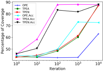
We consider industrial data on crystallization of ceramic thin films in [Nakamura et al., 2017]. The goal for the industrial application on crystallization of ceramic thin films is to determine an optimal setting for the volume of tetraethylene glycol (TEG), temperature (T), and the time of heat to a temperature in time (HTI), which is in fact a SZCO problem. The objective of the experiment is a quadratic function. For more details, please refer to [Nakamura et al., 2017; Wang et al., 2017].
By updating the values of TEG, T and HTI, we show the growth of ceramic thin films with the number of iterations in Figure 2. The superior performance of the acceleration via Algorithm 1 is clear. We also test different intensity of noises, and find that the acceleration is robust. Note that, in ceramic thin films, we solve a concave function and thus the function value increases.
5 Conclusions
In this paper, we have developed a generic acceleration approach to solve the problem of SZCO. We tackled the SZCO problem with the core idea of exploring an LEB condition of objective functions, which is frequently encountered in real applications. The benefits of the proposed acceleration technique are three-fold: wide applicability, weak assumption and improvements on iteration complexity. With LEB condition, the best upper bound here can be min(O(d2 log(1/ϵ)), ˜O(d/ϵ)), and the improvement over existing results is up to a factor of 1/ϵ2 . Experimental results have shown superior and robust performance of the proposed acceleration approach.
Acknowledgments
The work described in this paper was partially supported by the Research Grants Council of the Hong Kong Special Administrative Region, China (No. CUHK 14208815 and No. CUHK 14234416 of the General Research Fund), Microsoft Research Asia (2018 Microsoft Research Asia Collaborative Research Award), and National Science Foundation (NSF1545995). Part of X. Yu's work was conducted at the University of Iowa when visiting T. Yang's research group.
@inproceedings{ijcai2018p422,
  title     = {A Generic Approach for Accelerating Stochastic Zeroth-Order Convex Optimization},
  author    = {Yu, Xiaotian and King, Irwin and Lyu, Michael R. and Yang, Tianbao},
  booktitle = {Proceedings of the Twenty-Seventh International Joint Conference on
               Artificial Intelligence, {IJCAI-18}},
  publisher = {International Joint Conferences on Artificial Intelligence Organization},
  editor    = {Jérôme Lang},
  pages     = {3040--3046},
  year      = {2018},
  month     = {7},
  note      = {Main track},
  doi       = {10.24963/ijcai.2018/422},
  url       = {https://doi.org/10.24963/ijcai.2018/422},
}
TY - CPAPER TI - A Generic Approach for Accelerating Stochastic Zeroth-Order Convex Optimization AU - Yu, Xiaotian AU - King, Irwin AU - Lyu, Michael R. AU - Yang, Tianbao T2 - Proceedings of the Twenty-Seventh International Joint Conference on Artificial Intelligence, IJCAI-18 PB - International Joint Conferences on Artificial Intelligence Organization PY - 2018 SP - 3040 EP - 3046 DO - 10.24963/ijcai.2018/422 UR - https://doi.org/10.24963/ijcai.2018/422 ER -Copied
Machine-readable versions of this paper, for tools and AI agents:





