
Towards Enabling Binary Decomposition for Partial Label Learning
Proceedings of the Twenty-Seventh International Joint Conference on Artificial Intelligence. Main track. Pages 2868-2874.
https://doi.org/10.24963/ijcai.2018/398
Keywords
- Machine Learning: Multi-instance;Multi-label;Multi-view learning
- Machine Learning: Classification
Abstract
The task of partial label (PL) learning is to learn a multi-class classifier from training examples each associated with a set of candidate labels, among which only one corresponds to the ground-truth label. It is well known that for inducing multi-class predictive model, the most straightforward solution is binary decomposition which works by either one-vs-rest or one-vs-one strategy. Nonetheless, the ground-truth label for each PL training example is concealed in its candidate label set and thus not accessible to the learning algorithm, binary decomposition cannot be directly applied under partial label learning scenario. In this paper, a novel approach is proposed to solving partial label learning problem by adapting the popular one-vs-one decomposition strategy. Specifically, one binary classifier is derived for each pair of class labels, where PL training examples with distinct relevancy to the label pair are used to generate the corresponding binary training set. After that, one binary classifier is further derived for each class label by stacking over predictions of existing binary classifiers to improve generalization. Experimental studies on both artificial and real-world PL data sets clearly validate the effectiveness of the proposed binary decomposition approach w.r.t state-of-the-art partial label learning techniques.
- [Amores, 2013] J. Amores. Multiple instance classification: Review, taxonomy and comparative study. Artificial Intel- ligence, 201:81-105, 2013.
- [Bache and Lichman, 2013] K. Bache and M. Lichman. U- CI machine learning repository. School of Information and Computer Sciences, University of California, Irvine, 2013.
- [Briggs et al., 2012] F. Briggs, X. Z. Fern, and R. Raich. Rank-loss support instance machines for MIML instance annotation. In Proceedings of the 18th ACM SIGKDD In- ternational Conference on Knowledge Discovery and Data Mining, pages 534-542, Beijing, China, 2012.
- [Chang and Lin, 2011] C. C. Chang and C. J. Lin. Libsvm: a library for support vector machines. ACM Transactions on Intelligent Systems and Technology, 2(3):27, 2011.
- [Chen et al., 2014] Y.-C. Chen, V. M. Patel, R. Chellappa, and P. J. Phillips. Ambiguously labeled learning using dic- tionaries. IEEE Transactios on Information Forensics and Security, 9(12):2076-2088, 2014.
- Chen et al., in press] C.-H. Chen, V. M. Patel, and R. Chel- lappa. Learning from ambiguously labeled face images. IEEE Transactions on Pattern Analysis and Machine In- telligence, in press.
- [Cour et al., 2011] T. Cour, B. Sapp, and B. Taskar. Learn- ing from partial labels. Journal of Machine Learning Re- search, 12(May):1501-1536, 2011.
- [Dietterich and Bakiri, 1995] T. G. Dietterich and G. Bakiri. Solving multiclass learning problem via error-correcting output codes. Journal of Artificial Intelligence Research, 2(1):263-286, 1995.
- [Gong et al., 2018] C. Gong, T. Liu, Y. Tang, J. Yang, J. Yang, and D. Tao. A regularization approach for instance-based superset label learning. IEEE Transactions on Cybernetics, 48(3):967-978, 2018.
- [Guillaumin et al., 2010] M. Guillaumin, J. Verbeek, and C. Schmid. Multiple instance metric learning from au- tomatically labeled bags of faces. In Lecture Notes in Computer Science 6311, pages 634-647. Springer, Berlin, 2010.
- [Hüllermeier and Beringer, 2006] E. Hüllermeier and J. Beringer. Learning from ambiguously labeled ex- amples. Intelligent Data Analysis, 10(5):419-439, 2006.
- [Jie and Orabona, 2010] L. Jie and F. Orabona. Learning from candidate labeling sets. In Advances in Neural In- formation Processing Systems 23, pages 1504-1512. MIT Press, Cambridge, MA, 2010.
- [Jin and Ghahramani, 2003] R. Jin and Z. Ghahramani. Learning with multiple labels. In Advances in Neural In- formation Processing Systems 15, pages 897-904. MIT Press, Cambridge, MA, 2003.
- [Liu and Dietterich, 2012] L. Liu and T. Dietterich. A condi- tional multinomial mixture model for superset label learn- ing. In Advances in Neural Information Processing Sys- tems 25, pages 557-565. MIT Press, Cambridge, MA, 2012.
- [Nguyen and Caruana, 2008] N. Nguyen and R. Caruana. Classification with partial labels. In Proceedings of the 14th ACM SIGKDD International Conference on Knowl- edge Discovery and Data Mining, pages 381-389, Las Ve- gas, NV, 2008.
- [Panis and Lanitis, 2015] G. Panis and A. Lanitis. An overview of research activities in facial age estimation us- ing the fg-net aging database. In Lecture Notes in Comput- er Science 8926, pages 737-750. Springer, Berlin, 2015.
- [Tang and Zhang, 2017] C.-Z. Tang and M.-L. Zhang. Confidence-rated discriminative partial label learning. In Proceedings of the 31st AAAI Conference on Artificial In- telligence, pages 2611-2617, San Francisco, CA, 2017.
- [Yu and Zhang, 2017] F. Yu and M.-L. Zhang. Maxi- mum margin partial label learning. Machine Learning, 106(4):573-593, 2017.
- [Zeng et al., 2013] Z. Zeng, S. Xiao, K. Jia, T.-H. Chan, S. Gao, D. Xu, and Y. Ma. Learning by associating am- biguously labeled images. In Proceedings of the IEEE Computer Society Conference on Computer Vision and Pattern Recognition, pages 708-715, Portland, OR, 2013.
- [Zhang and Yu, 2015] M.-L. Zhang and F. Yu. Solving the partial label learning problem: An instance-based ap- proach. In Proceedings of the 24th International Join- t Conference on Artificial Intelligence, pages 4048-4054, Buenos Aires, Argentina, 2015. IJCAI
- [Zhang and Zhou, 2014] M.-L. Zhang and Z.-H. Zhou. A re- view on multi-label learning algorithms. IEEE Transac- tions on Knowledge and Data Engineering, 26(8):1819- 1837, 2014.
- [Zhang et al., 2017] M.-L. Zhang, F. Yu, and C.-Z. Tang. Disambiguation-free partial label learning. IEEE Transac- tions on Knowledge and Data Engineering, 29(10):2155- 2167, 2017.
- [Zhou, 2012] Z.-H. Zhou. Ensemble Methods: Foundations and Algorithms. Chapman & Hall/CRC, Boca Raton, FL, 2012.
- Zhou, in press] Z.-H. Zhou. A brief introduction to weakly supervised learning. National Science Review, in press.
- [Zhu and Goldberg, 2009] X. Zhu and A. B. Goldberg. Intro- duction to semi-supervised learning. In Synthesis Lectures to Artificial Intelligence and Machine Learning, pages 1- 130.
References were extracted automatically from the PDF and may contain errors.
Full text extracted automatically from the PDF; figures, tables and equations may differ. The PDF is the version of record.
1 Introduction
In partial label (PL) learning, each training example is represented by a single instance while associated with a set of candidate labels, among which only one label is valid [Cour et al., 2011; Chen et al., 2014; Yu and Zhang, 2017]. Partial label learning has manifested its capability in solving real-world problems where only weakly-supervised information can be acquired, such as web mining [Jie and Orabona, 2010], multimedia contents analysis [Zeng et al., 2013; Chen et al., in press], ecoinformatics [Liu and Dietterich, 2012; Tang and Zhang, 2017], etc.
∗This work was supported by the National Key R&D Program of China (SQ2018YFB100002), the National Science Foundation of China (61573104), the Fundamental Research Funds for the Central Universities (2242018K40082), and partially supported by the Collaborative Innovation Center of Novel Software Technology and Industrialization.
†Corresponding author
Formally speaking, let X = Rd be the d-dimensional instance space and Y = {λ1, λ2, . . . , λq} be the label space with q class labels. Given a set of PL training examples D = {(xi, Si)|1 ≤ i ≤ m}, partial label learning aims to induce a multi-class classification model f : X ↦→ Y from D. Here, xi ∈ X is a d-dimensional feature vector (xi1, xi2, . . . , xid)T and Si ⊆ Y is the associated candidate label set. Following the key assumption of partial label learning, the ground-truth label yi for xi is concealed in its candidate label set (i.e. yi ∈ Si) and therefore cannot be accessed by the learning algorithm.
To accomplish the task of learning from partial label data, a number of approaches have been proposed by fitting widely-used learning techniques to partial label data, such as k-nearest neighbor [H¨ullermeier and Beringer, 2006; Zhang and Yu, 2015; Gong et al., 2018], maximum margin [Nguyen and Caruana, 2008; Yu and Zhang, 2017], maximum likelihood [Jin and Ghahramani, 2003; Liu and Dietterich, 2012], boosting [Tang and Zhang, 2017], etc. However, other than fitting existing learning techniques to data, a natural postulation is that whether partial label learning problem can be solved by fitting data to existing learning techniques. Specifically, considering that the ultimate goal of partial label learning is to induce a multi-class classifier, binary decomposition should serve as the most straightforward solution for fulfilling multi-class classification. Unfortunately, due to the fact that ground-truth label is not accessible from the PL training example, neither the one-vs-rest nor the one-vs-one binary decomposition strategy can be directly employed under partial label learning scenario.
In this paper, we aim to enable binary decomposition for partial label learning by adapting the popular one-vs-one decomposition strategy. Accordingly, a novel partial label learning algorithm named PALOC, i.e. PAtial Label learning via One-vs-one deComposition, is proposed. During the training phase, one binary classifier is derived for each pair of class labels, where PL training examples which have distinct relevancy to the label pair are utilized to instantiate the corresponding binary training set. Furthermore, an auxiliary set of binary classifiers (one per class label) are derived by stacking over the predictive outputs of existing binary classifiers to help improve generalization. During the test phase, classification results yielded by all binary classifiers are synergized to make prediction on unseen instance. Extensive experiments on artificial as well as real-world PL data sets clearly show that PALOC achieves highly competitive performance against state-of-the-art partial label learning approaches.
The rest of this paper is organized as follows. Section 2 presents technical details of the proposed PALOC approach. Section 3 discusses existing works related to PALOC. Section 4 reports detailed results of comparative experiments. Finally, Section 5 concludes.
2 The PALOC Approach
Following the notations given in Section 1, partial label learning aims to induce a multi-class classifier f : X ↦→ Y fromD which maps from the instance space to the label space. Generally, binary decomposition serves as an intuitive solution which transforms multi-class learning problem into a number of binary learning problems. The main difficulty of applying binary decomposition techniques to partial label learning lies in that the ground-truth label yi of each PL training example (xi, Si) is concealed in its candidate label set Si. Thereafter, for the one-vs-rest binary decomposition strategy, it is unclear whether (xi, Si) should be regarded as a positive or negative example w.r.t. one specific class label. For the one-vs-one binary decomposition strategy, it is unclear which class label should (xi, Si) belong to w.r.t. a pair of class labels.
PALOC enables binary decomposition for partial label learning by fitting PL data to the one-vs-one (OVO) decomposition strategy. Specifically, for each pair of class labels (λj, λk), the relevancy of (xi, Si) to λj and λk is determined via their assignment to the candidate label set instead of their equivalence to the (unknown) ground-truth label. Let ¯ Si = Y \ Si denote the complementary label set of Si in Y, a binary training set is constructed w.r.t. each pair of class labels (λj, λk) as follows:
In other words, only PL training example (xi, Si) where λj and λk have distinct assignment to Si is utilized to instantiate the binary training set Djk. Accordingly, a binary classifier gjk : X ↦→ R is derived by invoking some binary training algorithmB on Djk, i.e. gjk ←[B(Djk). Without loss of generality, a total of (q2) can be derived from the above one-vs-one binary decomposition procedure (by assuming j < k). Furthermore, each PL training example (xi, Si) will contribute to the learning procedure of |Si|| ¯ Si| binary classifiers.
Given the set of (q2) binary classifiers, the class label for any instance x can be predicted by counting the votes yielded by all classifiers:
Although it is feasible to make final prediction based on Eq.(2), PALOC employs stacking strategy [Zhou, 2012] to further improve generalization performance. For each PL training example (xi, Si), its candidate label set Si can be refined to ˆ Si as follows:
Here, ˆ yi = arg maxλj∈Y Vovo(xi, λj ) corresponds to the disambiguation prediction for xi based on Eq.(2). Therefore, the candidate label set is refined to be {ˆ yi} if the disambiguation prediction falls into Si. Otherwise, the candidate label set remains unchanged.
Given the set of (q2) binary classifiers gjk (1 ≤ j < k ≤ q), an auxiliary set of q binary classifiers (one per class label) are further derived via stacked generalization. For each class label λj (1 ≤ j ≤ q), a corresponding binary training set is constructed as follows:
In other words, for each binary training example in Dj, ˆxi is formed by augmenting the original feature vector xi with the predictive outputs of all (q2) classifiers. Furthermore, the binary label φ( ˆ Si, λj) is determined by the assignment of λj w.r.t. the refined candidate label set ˆ Si. Accordingly, a binary classifier gj : X ↦→ R is further derived by invoking some binary training algorithm B on Dj , i.e. gj ←[B(Dj).
During the testing phase, the unseen instance x∗ is firstly fed to the (q2) classifiers to generate the augmented feature vector:
After that, the set of (q2) classifiers gjk (1 ≤ j < k ≤ q) and the other set of q classifiers gj (1 ≤ j ≤ q) are synergized to make prediction on x∗ :
Here, µ is the balance parameter which controls the relative importance of Vovo(x∗ , λj), i.e. the votes yielded by onevs-one binary classifiers, and Vstack(x∗ , λj), i.e. the votes yielded by stacking binary classifiers.
Inputs:
- D:
- the partial label training set {(xi, Si) | 1 ≤ i ≤ m} (xi ∈ X , Si ⊆ Y, X = Rd , Y = {λ1, λ2, . . . , λq})
- B: binary training algorithm
- µ: the balance parameter
- x∗ : the unseen instance
Outputs:
y∗ : the predicted class label for x∗
Process:
- 1: for j = 1 to q -1 do
- 2: for k = j + 1 to q do
- 3: Construct the one-vs-one binary training set Djk according to Eq.(1);
- 4: gjk ←[B(Djk);
- 5: end for
- 6: end for
- 7: for i = 1 to mdo
- 8: Obtain the disambiguation prediction ˆ yi for xi according to Eq.(2);
- 9: Identify the refined candidate label set ˆ Si for xi according to Eq.(3);
- 10: end for
- 11: for j = 1 to q do
- 12: Construct the stacking binary training set Dj according to Eq.(4);
- 13: gj ←B(Dj);
- 14: end for
- 15: Generate the augmented feature vector ˆx∗ for x∗ according to Eq.(5);
- 16: Return y∗ = f(x∗ ) according to Eq.(6).
Table 1: The pseudo-code of PALOC.
Table 1 summarizes the complete procedure of the proposed PALOC approach. Given the partial label training set, binary training sets are constructed by adapting one-vs-one decomposition strategy and then utilized to induce (q2) binary classifiers (Steps 1-6). After that, the derived binary classifiers are employed to augment the feature vector and refine the candidate label set of PL training examples (Steps 7-10). Accordingly, a set of q binary classifiers are further constructed based on the stacking strategy (Steps 11-14). Finally, the unseen instance is classified by referring to the predictive outputs of all the binary classifiers (Steps 15-16).
3 RelatedWork
Partial label learning deals with weak supervision information where the labeling information of each PL training example is implicit and not accessible to the learning algorithm. Generally, partial label learning is related to several wellestablished weakly-supervised learning frameworks such as semi-supervised learning, multi-instance learning and multilabel learning. Nonetheless, different weak supervision scenarios are considered by those learning frameworks [Zhou, in press].
Semi-supervised learning [Zhu and Goldberg, 2009] aims to induce a classifier f : X ↦→ Y from both labeled and unlabeled examples, where the ground-truth label assumes the whole label space for unlabeled example while assumes the candidate label set for PL example. Multi-instance learning [Amores, 2013] aims to induce a classifier f : 2X ↦→ Y from examples each represented as a labeled bag of instances, where a single label is assigned to a set of instances for multiinstance example while a set of labels are assigned to a single instance for PL example. Multi-label learning [Zhang and Zhou, 2014] aims to induce a classifier f : X ↦→ 2Y from training examples each associated with multiple labels, where the associated labels are all valid ones for multi-label example while the associated labels are only candidate ones for PL example.
Most existing algorithms learn from PL examples by fitting widely-used learning techniques to partial label data. For maximum likelihood techniques, the likelihood of observing each PL training example is defined over its candidate label set instead of the unknown ground-truth label [Jin and Ghahramani, 2003; Liu and Dietterich, 2012]. For k-nearest neighbor techniques, the candidate label sets of neighboring instances are merged via weighted voting for making prediction [H¨ullermeier and Beringer, 2006; Zhang and Yu, 2015]. For maximum margin techniques, the classification margin over each PL training example is defined by discriminating modeling outputs from candidate labels and non-candidate labels [Nguyen and Caruana, 2008; Yu and Zhang, 2017]. For boosting techniques, the weight over each PL training example and the confidence of each candidate label being the ground-truth label are updated in each boosting round [Tang and Zhang, 2017].
Other than fitting existing learning techniques to PL data, there are few works which work by fitting PL data to existing learning techniques. The CLPL approach [Cour et al., 2011] maps a d-dimensional instance in X into a d×q-dimensional feature vector for each class label in Y. For each PL training example (xi, Si), one positive example is generated by averaging mapped feature vectors w.r.t. candidate labels in Si and q - |Si| negative examples are generated by taking the mapped feature vector w.r.t. each non-candidate label in Y \ Si. The PL-ECOC approach [Zhang et al., 2017] transforms each instance into a binary example based on the utilization of ECOC coding matrix [Dietterich and Bakiri, 1995; Zhou, 2012]. For each PL training example (xi, Si), it is regarded as a positive or negative example if its candidate label set Si entirely falls into the column dichotomy of the coding matrix. Although both CLPL and PL-ECOC work by transforming the partial label learning problem into binary learning problem, PALOC enables binary decomposition for PL data in a more concise manner without relying on extra manipulations such as feature mapping or coding matrix.
4 Experiments
4.1 Comparing Algorithms
To evaluation the performance of PALOC, five state-of-the-art partial label learning approaches with suggested parameter configurations have been employed for comparative studies:
- CLPL [Cour et al., 2011] which transforms partial label learning problem to binary learning problem via feature mapping with convex loss optimization [suggested configuration: SVMwith squared hinge loss];
- PL-KNN [H¨ullermeier and Beringer, 2006] which adapts k-nearest neighbor technique to learn from PL data via weighted voting [suggested configuration: k = 10];
- PL-SVM [Nguyen and Caruana, 2008] which adapts maximum margin technique to learn from PL data via l2 regularization [suggested configuration: regularization parameter pool with {10-3 , . . . , 103 }];
- LSB-CMM [Liu and Dietterich, 2012] which adapts maximum likelihood to learn from PL data via mixture models [suggested configuration: 5q mixture components];
- PL-ECOC [Zhang et al., 2017] which transforms partial label learning problem to binary learning problem via ECOC coding matrix [suggested configuration: codeword length L = ⌈10 log2(q)⌉].
As shown in Table 1, the only parameter to be set for PALOC is µ, which controls relative importance of the generated one-vs-one classifiers and stacking classifiers. In the rest of this paper, µ is fixed to be 10 for performance evaluation. Furthermore, similar to CLPL and PL-ECOC, SVM [Chang and Lin, 2011] is utilized to instantiate the binary base learner B for PALOC.
Next, two series of experiments are conducted on controlled UCI data sets as well as real-world partial label data Configurations
| Data Set | #Examples | #Features | #Class Labels |
|---|---|---|---|
| glass | 214 | 10 | 5 |
| ecoli | 336 | 7 | 8 |
| vehicle | 846 | 18 | 4 |
| abalone | 4,177 | 7 | 29 |
| usps | 9,298 | 256 | 10 |
| letter | 20,000 | 16 | 26 |
(I) r = 1, p ∈ {0.1, 0.2, . . . , 0.7}
(II) r = 2, p ∈ {0.1, 0.2, . . . , 0.7}
(III) r = 3, p ∈ {0.1, 0.2, . . . , 0.7}
(IV) p = 1, r = 1, ϵ ∈ {0.1, 0.2, . . . , 0.7}
Table 2: Characteristics of the controlled UCI data sets.
sets. For each data set, ten-fold cross-validation is performed where the mean predictive accuracies and standard deviations are recorded for all comparing approaches.
4.2 Controlled UCI Data Sets
Table 2 summarizes the characteristics of six controlled UCI data sets [Bache and Lichman, 2013]. Concretely, following the widely-used controlling protocol, an artificial partial label data set is generated from one multi-class UCI data set under specified configuration of three controlling parameters p, r and ϵ [Cour et al., 2011; Liu and Dietterich, 2012; Chen et al., 2014; Zhang et al., 2017]. Here, p controls the proportion of examples which are partially labeled (i.e. |Si| > 1), r controls the number of false positive labels in the candidate label set (i.e. |Si| = r + 1), and ϵ controls the co-occurring probability between one extra candidate label and the groundtruth label. As shown in Table 2, a total of 28 (4x7) parameter configurations are considered for each controlled UCI data set.
| PALOC against | |||||
|---|---|---|---|---|---|
| CLPL | PL-KNN | PL-SVM | LSB-CMM | PL-ECOC | |
| varying p [r=1] | 35/7/0 | 28/14/0 | 34/8/0 | 25/16/1 | 7/30/5 |
| varying p [r=2] | 30/12/0 | 29/13/0 | 32/10/0 | 22/20/0 | 7/30/5 |
| varying p [r=3] | 35/7/0 | 31/11/0 | 37/5/0 | 21/21/0 | 9/29/4 |
| varying ϵ [p, r=1] | 22/15/5 | 30/9/3 | 29/13/0 | 22/18/2 | 10/26/6 |
| In Total | 122/41/5 | 118/47/3 | 132/36/0 | 90/75/3 | 33/115/20 |
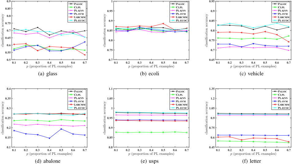
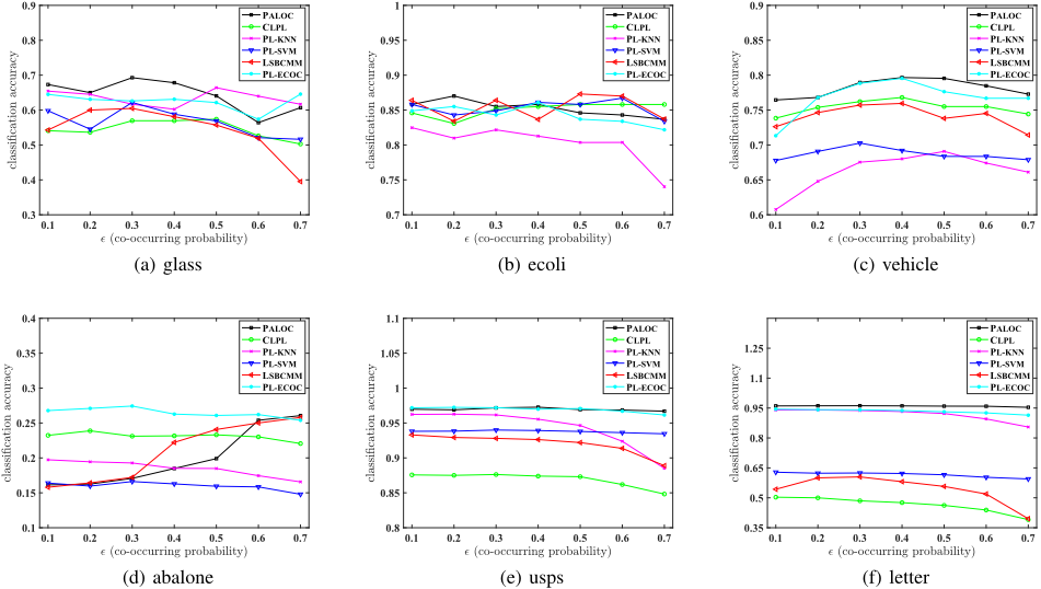
Figure 1 illustrates the classification accuracy of each comparing algorithm as p increases from 0.1 to 0.7 with step-size 0.1 (r = 1). Along with the ground-truth label, one class label in Y will be randomly picked up to constitute the candidate label set. Due to page limit, figures for the cases of r = 2 and r = 3 are not illustrated here while similar results to Figure 1 can be observed as well. Figure 2 illustrates the classification accuracy of each comparing algorithm as ϵ increases from 0.1 to 0.7 with step-size 0.1 (p = 1, r = 1). Given any label λ ∈ Y, one extra label λ′ ∈ Y is designated as the coupling label which co-occurs with λ in the candidate label set with probability ϵ. Otherwise, any other class label would be randomly chosen to co-occur with λ.
As illustrated in Figures 1 and 2, the performance of PALOC is highly competitive to other comparing algorithms in most cases. Furthermore, pairwise t-test at 0.05 significance level is conducted based on the results of ten-fold cross-validation. Table 3 reports the win/tie/loss counts between PALOC and each comparing approach. Specifically, out of the 168 statistical tests (28 configurations x 6 UCI data sets), it is shown that: 1) PALOC achieves superior or at least comparable performance against PL-SVM in all cases; 2) PALOC achieves superior performance against PL-KNN and LSB-CMM in 70.2% and 53.6% cases while has been outperformed by either of them in only 1.8% cases; 3) PALOC achieves superior performance against CLPL and PL-ECOC in 72.6% and 19.6% cases while has been outperformed by them in only 3.0% and 11.9% cases respectively.
| Data Set | #Examples | #Features | #Class Labels | avg. #CLs | Task Domain |
|---|---|---|---|---|---|
| 1,002 | 262 | 78 | 7.48 | facial age estimation [Panis and Lanitis, 2015] | FG-NET |
| Lost 1,122 | 108 | 16 | 2.23 automatic et al., 2011] | face naming [Cour | |
| MSRCv2 1,758 | 48 | 23 | 3.16 | object classification [Liu and Dietterich, 2012] | |
| 4,998 | 38 | 13 | 2.18 song classification [Briggs et al., 2012] | BirdSong bird | |
| Soccer Player 17,472 | 279 | 171 | 2.09 | automatic face naming [Zeng et al., 2013] | |
| Yahoo! News 22,991 | 163 | 219 | 1.91 | automatic face naming [Guillaumin et al., 2010] |
| FG-NET | Lost | MSRCv2 | BirdSong | Soccer Player | Yahoo! News | |
|---|---|---|---|---|---|---|
| PALOC | 0.065±0.019 | 0.629±0.056 | 0.479±0.042 | 0.711±0.016 | 0.537±0.015 | 0.625±0.005 |
| CLPL | 0.063±0.027 | 0.742±0.038◦ | 0.413±0.041• | 0.632±0.019• | 0.368±0.010• | 0.462±0.009• |
| PL-KNN | 0.038±0.025• | 0.424±0.036• | 0.448±0.037• | 0.614±0.021• | 0.497±0.015• | 0.457±0.004• |
| PL-SVM | 0.063±0.029 | 0.729±0.042◦ | 0.461±0.046 | 0.660±0.037• | 0.464±0.011• | 0.629±0.010 |
| LSB-CMM | 0.059±0.025 | 0.693±0.035◦ | 0.473±0.037 | 0.672±0.056 | 0.498±0.017• | 0.645±0.005◦ |
| PL-ECOC | 0.040±0.018• | 0.653±0.053 | 0.440±0.039 | 0.731±0.013◦ | 0.494±0.015• | 0.610±0.009• |
4.3 Real-World Data Sets
Table 4 summarizes the characteristics of real-world partial label data sets, which are collected from several application domains including FG-NET [Panis and Lanitis, 2015] for facial age estimation, Lost [Cour et al., 2011], Soccer Player [Zeng et al., 2013] and Yahoo!News [Guillaumin et al., 2010] for automatic face naming from images or videos, MSRCv2 [Liu and Dietterich, 2012] for object classification, and BirdSong [Briggs et al., 2012] for bird song classification. The average number of candidate labels (avg. #CLs) for each real-world partial label data set is also recorded in Table 4.
Table 5 reports the mean classification accuracy as well as standard deviation of each comparing algorithm. Pairwise t-test at 0.05 significance level is conducted based on the ten-fold cross-validation, where the test outcomes between PALOC and the comparing approaches are also recorded.
As shown in Table 5, it is impressive to observe that: 1) On all data sets, PALOC significantly outperforms PLKNN; 2) PALOC achieves superior performance or at least comparable performance to CLPL and PL-SVM on all data sets except Lost; 3) PALOC significantly outperforms PLECOC on FG-NET, Soccer Player and Yahoo!News, and achieves comparable performance to PL-ECOC on Lost and MSRCv2; 4) PALOC achieves superior performance or at least comparable performance to LSB-CMM on FG-NET, MSRCv2, BirdSong and Soccer Player.
4.4 Sensitivity Analysis
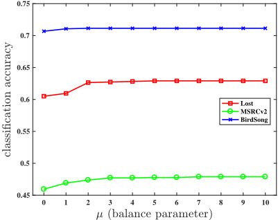
As shown in Eq.(6), PALOC employs parameter µ to balance the voting predictions from one-vs-one classifiers and stacking classifiers respectively. To investigate the performance sensitivity of PALOC w.r.t. µ, Figure 3 shows how the classification accuracy of PALOC changes as µ varies from 0 to 10 with step-size 1. Here, three real-world PL data sets Lost, MSRCv2 and BirdSong are employed for illustrative purpose. As shown in Figure 3, it is obvious that the performance of PALOC improves as µ increases from 0 and becomes relatively stable as µ reaches 4. Note that µ = 0 corresponds to the case where only one-vs-one classifiers contribute to the final prediction, and these observations indicate that the stacking classifiers do help improve the performance of PALOC.
5 Conclusion
In this paper, the problem of partial label learning is studied where a novel approach based on binary decomposition is proposed. Specifically, one-vs-one decomposition strategy is enabled to deal with partial label learning problem by considering the relevancy of each label pair w.r.t. the candidate label set of PL training examples. Effectiveness of the proposed approach is validated via comprehensive experiments on both controlled UCI data sets and real-world PL data sets.
As shown in Eq.(1), not all PL training examples will contribute to the construction of binary training set w.r.t. each label pair. Therefore, it is interesting to explore possible ways to make full use of the excluded PL training examples to further enhance the proposed binary decomposition approach.
@inproceedings{ijcai2018p398,
  title     = {Towards Enabling Binary Decomposition for Partial Label Learning},
  author    = {Wu, Xuan and Zhang, Min-Ling},
  booktitle = {Proceedings of the Twenty-Seventh International Joint Conference on
               Artificial Intelligence, {IJCAI-18}},
  publisher = {International Joint Conferences on Artificial Intelligence Organization},
  editor    = {Jérôme Lang},
  pages     = {2868--2874},
  year      = {2018},
  month     = {7},
  note      = {Main track},
  doi       = {10.24963/ijcai.2018/398},
  url       = {https://doi.org/10.24963/ijcai.2018/398},
}
TY - CPAPER TI - Towards Enabling Binary Decomposition for Partial Label Learning AU - Wu, Xuan AU - Zhang, Min-Ling T2 - Proceedings of the Twenty-Seventh International Joint Conference on Artificial Intelligence, IJCAI-18 PB - International Joint Conferences on Artificial Intelligence Organization PY - 2018 SP - 2868 EP - 2874 DO - 10.24963/ijcai.2018/398 UR - https://doi.org/10.24963/ijcai.2018/398 ER -Copied
Machine-readable versions of this paper, for tools and AI agents:





