
Accelerated Difference of Convex functions Algorithm and its Application to Sparse Binary Logistic Regression
Proceedings of the Twenty-Seventh International Joint Conference on Artificial Intelligence. Main track. Pages 1369-1375.
https://doi.org/10.24963/ijcai.2018/190
Keywords
- Constraints and SAT: Constraint Optimisation
- Machine Learning: Classification
- Machine Learning: Feature Selection ; Learning Sparse Models
Abstract
In this work, we present a variant of DCA (Difference of Convex function Algorithm) with the aim to improve its convergence speed. The proposed algorithm, named Accelerated DCA (ADCA), consists in incorporating the Nesterov's acceleration technique into DCA. We first investigate ADCA for solving the standard DC program and rigorously study its convergence properties and the convergence rate. Secondly, we develop ADCA for a special case of the standard DC program whose the objective function is the sum of a differentiable with L-Lipschitz gradient function (possibly nonconvex) and a nonsmooth DC function. We exploit the special structure of the problem to propose an efficient DC decomposition for which the corresponding ADCA scheme is inexpensive. As an application, we consider the sparse binary logistic regression problem. Numerical experiments on several benchmark datasets illustrate the efficiency of our algorithm and its superiority over well-known methods.
- [Attouch and Bolte, 2009] Hedy Attouch and Jerome Bolte. On the convergence of the proximal algorithm for nons- mooth functions involving analytic features. Mathematical Programming, 116(1):5-16, 2009.
- [Beck and Teboulle, 2009a] Amir Beck and Marc Teboulle. Fast gradient-based algorithms for constrained total vari- ation image denoising and deblurring problems. IEEE Transactions on Image Processing, 18(11):2419-2434, 2009.
- [Beck and Teboulle, 2009b] Amir Beck and Marc Teboulle. A fast iterative shrinkage-thresholding algorithm for lin- ear inverse problems. SIAM Journal on Imaging Sciences, 2:183-202, 2009.
- [Bradley and Mangasarian, 1998] Paul Bradley and Olvi Leon Mangasarian. Feature selection via concave minimization and support vector machines. In Machine Learning Proceedings of the Fifteenth International Conference (ICML '98), pages 82-90, 1998.
- [Chambolle et al., 1998] Antonin Chambolle, Ronald De- Vore, Nam-Yong Lee, and Bradley Lucier. Nonlinear wavelet image processing: variational problems, compres- sion, and noise removal through wavelet shrinkage. IEEE Transactions on Image Processing, 7(3):319-335, 1998.
- [Combettes and Wajs, 2005] Patrick Combettes and Valerie Wajs. Signal recovery by proximal forward-backward splitting. Multiscale Modeling & Simulation, 4(4):1168- 1200, 2005.
- [Daubechies et al., 2004] Ingrid Daubechies, Michel De- frise, and Christine De Mol. An iterative thresholding al- gorithm for linear inverse problems with a sparsity con- straint. Communications on Pure and Applied Mathemat- ics, 57(11):1413-1457, 2004.
- [Dempster et al., 1977] Arthur Dempster, Natalie Laird, and Donald Rubin. Maximum likelihood from incomplete data via the em algorithm. Journal of the Royal Statistical So- ciety, Serie B, 39(1):1-38, 1977.
- [Frankel et al., 2015] Pierre Frankel, Guillaume Garrigos, and Peypouquet Peypouquet. Splitting methods with vari- able metric for kurdyka-łojasiewicz functions and general convergence rates. Journal of Optimization Theory and Applications, 165(3):874-900, 2015.
- [Grippo and Sciandrone, 2002] Luigi Grippo and Marco Sciandrone. Nonmonotone globalization techniques for the barzilai-borwein gradient method. Computational Op- timization and Applications, 23(2):143-169, 2002.
- [Gu et al., 2018] Bin Gu, Zhouyuan Huo, and Heng Huang. Inexact proximal gradient methods for non-convexand non-smooth optimization. In 32th AAAI Conference on Artificial Intelligence AAAI-18, 2018.
- [Hale et al., 2008] Elaine Hale, Wotao Yin, and Yin Zhang. Fixed-point continuation for ℓ 1 -minimization: Methodol- ogy and convergence. SIAM Journal on Optimization, 19(3):1107-1130, 2008.
- [Le Thi and Pham Dinh, 2005] Hoai An Le Thi and Tao Pham Dinh. The DC (difference of convex functions) programming and DCA revisited with DC models of real world nonconvex optimization problems. Annals of Oper- ations Research, 133:23-46, 2005.
- [Le Thi and Pham Dinh, 2018] Hoai An Le Thi and Tao Pham Dinh. DC programming and DCA: thirty years of developments. Mathematical Programming, Special Is- sue: DC Programming -Theory, Algorithms and Appli- cations, 169(1):5-64, 2018.
- [Le Thi et al., 2015] Hoai An Le Thi, Tao Pham Dinh, Hoai Minh Le, and Xuan Thanh Vo. DC approximation approaches for sparse optimization. European Journal of Operational Research, 244(1):26-46, 2015.
- [Li and Lin, 2015] Huan Li and Zhouchen Lin. Accelerated proximal gradient methods for nonconvex programming. In Advances in Neural Information Processing Systems, pages 377-387, 2015.
- [Nesterov, 1983] Yurii Nesterov. A method of solving a convex programming problem with convergence rate O(1/k 2 ). Soviet Mathematics Doklady, 27:372-376, 1983.
- [Pham Dinh and Le Thi, 1997] Tao Pham Dinh and Hoai An Le Thi. Convex analysis approach to D.C. programming: Theory, algorithms and applications. Acta Mathematica Vietnamica, 22(1):289-355, 1997.
- [Pham Dinh and Le Thi, 2014] T. Pham Dinh and H. A. Le Thi. Recent advances in dc programming and dca. In Transactions on Computational Intelligence XIII, pages 1- 37, 2014.
- [Wright et al., 2009] Stephen Wright, Robert Nowak, and Mario Figueiredo. Sparse reconstruction by separable ap- proximation. IEEE Transactions on Signal Processing, 57(7):2479-2493, 2009.
- [Yao et al., 2017] Quanming Yao, James. Kwok, Fei Gao, Wei Chen, and Tie-Yan Liu. Efficient inexact proximal gradient algorithm for nonconvex problems. In Proceed- ings of the Twenty-Sixth International Joint Conference on Artificial Intelligence, pages 3308-3314, 2017. IJCAI
- [Yuille and Rangarajan, 2003] A. L. Yuille and A. Rangara- jan. The concave-convex procedure. Neural Computation, 15(4):915-936, 2003.
References were extracted automatically from the PDF and may contain errors.
Full text extracted automatically from the PDF; figures, tables and equations may differ. The PDF is the version of record.
1 Introduction
A standard DC (Difference of Convex functions) program is of the form
where G and H are lower semi-continuous proper convex functions on Rn . Such a function F is called a DC function while G and H are the DC components of F . Note that a convex constraint x ∈ C can be incorporated into the objective function F by using the indicator function on C, defined by χC = 0 if x ∈ C and χC = +∞ if x ̸∈ C. The DC program (1) plays a key role in optimization since almost nonconvex programs encountered in practice can be formulated/reformulated as a DC program.
DCA (DC Algorithm) for solving the DC program (1) was introduced in 1985 by Pham Dinh Tao and extensively developed by Le Thi Hoai An and Pham Dinh Tao since 1994 to become now classic and increasingly popular ([Le Thi and Pham Dinh, 2005; 2018; Pham Dinh and Le Thi, 1997;
2014] and references therein). The original key idea of DCA relies on the structure DC of the objective function. DCA works with the DC components G and H but not directly with the function F. The main idea of DCA is simple: each iteration l of DCA approximates the concave part -H by its affine majorization (that corresponds to taking yk ∈ ∂H(xk )) and computes xk+1 by solving the resulting convex problem.
DCA has been successfully applied to various nonconvex/nonsmooth programs thanks to its versatility, flexibility, robustness, inexpensiveness and their adaptation to specific structure of considered problems. It has been proved that with an appropriate DC decompositions and a suitably equivalent DC reformulations, DCA permits to recover most of standard methods in convex and nonconvex programming. Several well-known methods in Machine Learning such as Expectation-Maximization (EM) [Dempster et al., 1977], Successive Linear Approximation (SLA) [Bradley and Mangasarian, 1998], Iterative Shrinkage-Thresholding Algorithms (ISTA) [Chambolle et al., 1998], and Convex-Concave Procedure (CCCP) [Yuille and Rangarajan, 2003] are special cases of DCA. The readers are referred to the recent paper [Le Thi and Pham Dinh, 2018] for an extensive overview of thirty years of development of DCA.
Nowadays, especially with the Big Data explosion, it has been becoming more and more important to develop advanced optimization methods able to handle very large-scale problems. Motivated by the success of DCA on several nonconvex/nonsmooth programs to which it was proved to be more robust and more efficient than related standard methods, we aim to investigate a variant of DCA in order to improve its performance.
Paper's contribution: the contributions of this paper is multiples.
Firstly, we introduce Accelerated DCA (ADCA) for solving the standard DC program (1). In ADCA, we incorporate the Nesterov's acceleration technique into standard DCA in order to improve its performance. The idea of ADCA is different to the usual line search acceleration using Armijo type rule which can be computationally costly. The acceleration step in ADCA which consists in using an extrapolated point from the current iterate and the previous one, aims to find a point zk which is better than xk for the computation of xk+1 .
We then provide a rigorous argument to prove the interesting convergence properties of ADCA as well as the convergence rate under the Lojasiewicz assumption.
Secondly, we investigate ADCA for a special case of the standard DC program, namely the sum of two nonconvex function minimization problem
where f is a differentiable function with L-Lipschitz continuous gradient (possibly nonconvex) and r is a DC function. The problem (2) covers several nonconvex and nonsmooth problems arising from various fields such as machine learning, computational biology, signal processing, etc.
The problem (2) has been attracting attention of many researchers. Proximal gradient (PG) methods, which are also known as different names ISTA, fixed point iteration, forward-backward splitting (see e.g. [Daubechies et al., 2004; Beck and Teboulle, 2009b; Combettes and Wajs, 2005; Hale et al., 2008]), have been extensively developed for the convex case of (2), i.e., both f and r are convex. In [Nesterov, 1983], the author introduced the first accelerated proximal gradient (APG) method for solving (2) with f convex and r = 0. Later, Beck and Teboulle [Beck and Teboulle, 2009a; 2009b] extended it for the case where both f and r are convex. These algorithms exhibit a global convergence rate O(1/k2 ), where k is the iteration counter. Recently, several extensions of APG method for the convex case of (2) have been proposed for the nonconvex cases. For instance, [Li and Lin, 2015] have extended the method of [Beck and Teboulle, 2009a] for f differentiable with L-Lipschitz gradient and r nonconvex. In [Gu et al., 2018], the authors presented inexact versions of PG and APG for solving (2) with f smooth and r nonsmooth (possibly nonconvex). Another inexact APG for the nonconvex case of (2) which only requires one proximal step at each iteration, were proposed in [Yao et al., 2017]. However, the aforementioned algorithms have to compute the proximal map of nonconvex functions r which do not has closed form in many cases. Usually, this computation can be very expensive or impossible.
In this work, by exploiting the properties of f and r, we propose an efficient DC decomposition for which the corresponding DCA and ADCA are inexpensive.
Finally, as an application, we consider the sparse binary logistic regression and carefully perform numerical experiments of all proposed algorithms.
The remainder of the paper is organized as follows. In Section 2 we introduce ADCA for the standard DC program and study its convergence properties. ADCA for solving the problem (2) is presented in Section 3. The numerical experiments on the sparse binary logistic regression problem are reported in Section 4 and Section 5 concludes the paper.
2 Accelerated DCA for Standard DC Program
Before presenting the Accelerated DCA, let us recall some basis notations that will be used in the sequel.
The modulus of strong convexity of θ on Ω, denoted by µ(θ, Ω) or µ(θ) if Ω = Rn , is given by
One says that θ is strongly convex on Ω if µ(θ, Ω) > 0.
For a convex function θ, the subdifferential of θ at x0 ∈ domθ := {x ∈ Rn : θ(x0) < +∞}, denoted by ∂θ(x0), is defined by
The subdifferential ∂θ(x0) generalizes the derivative in the sense that θ is differentiable at x0 if and only if ∂θ(x0) ≡ {∇xθ(x0)}.
A point x∗ is called a critical point of G-H, or a generalized Karush-Kuhn-Tucker point (KKT) of (Pdc)) if
We now introduce the Accelerated DCA (ADCA) for solving the standard DC program (1). According to the DCA scheme, at each iteration, one computes yk ∈ ∂H(xk ) then solves the convex sub-problem (1) to get xk+1 . The idea of ADCA, in order to accelerate DCA, is to find a point zk which is better than xk for the computation of xk+1 . In this work, we consider zk as an extrapolated point of the current iterate xk and the previous iterate xk-1 :
where tk+1 = 1+√1+4t2k 2 . If zk is better than one of last q iterates {xk-q , . . . , xk-1 , xk } in term of objective function, i.e., F(zk ) ≤ max t=max(0,k-q),...,k F(xt ) then zk will be used
instead of xk to compute yk . This condition allows the objective function F to increase and consequently to escape from a potential bad local minimum [Grippo and Sciandrone, 2002; Wright et al., 2009]. Theoretically, a large value of q increases the chance of using the extrapolated points zk in ADCA and consequently increases its chance to accelerate. Note that if q = 0 then F (zk ) ≤ F (xk ) and ADCA is a monotone algorithm like DCA. ADCA is described in Algorithm 1.
Algorithm 1 ADCA for solving the standard DC program (1)
Initialization: Choose an initial point x0 , z0 = x0 , q ∈ N, t0 = 1, and k ← 0.
repeat
- 2 2: Compute zk = xk + tk-1 tk+1 (xk - xk-1 ) if k ≥ 1.
- 1: Compute tk+1 = 1+√1+4t2k .
- 3: If F(zk ) ≤ maxt=max(0,k-q),...,k F(xt ) then set vk = zk , otherwise set vk = xk .
- 4: Compute yk ∈ ∂H(vk ).
- 5: Compute xk+1 = arg minx∈Rn {G(x) - 〈yk , x〉} .
- 6: k ← k + 1.
until Stopping criterion.
Remark 1. ADCA does not require any particular property of the sequence {tk} for extrapolation. The above sequence t was chosen thanks to its interesting convergence rate proved in [Beck and Teboulle, 2009b]. More precisely, the wellknown FISTA algorithm [Beck and Teboulle, 2009b] for solving the convex case of (2), i.e. both f(x) and r(x) are convex, is nothing else but a special case of ADCA in which we always use the extrapolated point zk instead of the last iterate xk . In FISTA, the extrapolated point vk is updated with tk+1 = 1+√1+4t2k 2 and the authors have proved that FISTA has a interesting convergence rate O( 1
k2 ).
2.1 Convergence Analysis of ADCA
In this subsection, we study the convergence of ADCA. Our first result provides the behavior of the limit points of the sequence {xφ(k) } generated by ADCA, where φ(k) = argmint=k+1,...,k+1+q ‖xt - vt-1 ‖2 .
Theorem 1. Let µ(G) and µ(H) be the convex modulus of G and H, respectively. If α = infx∈Rn F(x) > -∞ and min{µ(G), µ(H)} > 0, then for any subsequence {xφ(kj) } of {xφ(k) }, converging to x∗ such that {yφ(kj )-1 } is bounded, the limit point x∗ is a critical point of (1).
To prove Theorem 1, we will use the following lemma. Denote by {Γk } the sequence defined as
Lemma 1. Let {xk } and {vk } be sequences generated by ADCA. The following statements hold.
(i) For any k = 0, 1, ...,
As a result, by choosing q = 0, we get the monotone property of {F(xk )}, i.e., F(xk ) - F(xk+1 ) ≥ µ(G)+µ(H) 2 ‖xk+1 - vk ‖2 .
(ii) If α = infx∈Rn F (x) > -∞ and min{µ(G), µ(H)} > 0, then ∑+∞ k=0 ‖xφ(k) - vφ(k)-1 ‖2 < +∞, and therefore limk→+∞ ‖xφ(k) - vφ(k)-1 ‖ = 0.
Proof. First let us justify (i) by noting from the µ-convexity of G and yk ∈ ∂G(xk+1 ) that
It follows from the µ-convexity of H and yk ∈ ∂H(vk ) that
Summing two above inequalities gives us
Observe that F(vk ) ≤ maxt=max(0,k-d),...,k F(xt ) = Γk . It follows from this and (5) that
This implies that F(xk+1 ) ≤ Γk . We prove by induction that for all t = 0, ..., q
Indeed, it follows from (6) that the claim holds for t = 0. We suppose that it also holds for t = 0, ..., p - 1 with 1 ≤ p ≤ q. Thus, we have
where last inequality follows from F(xk+1+t ) ≤ Γk for t = 0, ..., p - 1. Therefore, we obtain
Next let us prove (ii) by noting that Γk ≥ α for all k. Summing (4) over k = 0, ..., N gives us that
Since min{µ(G), µ(H)} > 0, we have
Passing to the limit over the sequence {N}N∈N tells us that
Proof of Theorem 1. Let {xφ(kj) } be a subsequence of {xφ(k) } that converges to x∗ . It follows from (ii) of Lemma 1 that limj→+∞ vφ(kj)-1 = x∗ . Without loss of generality, we can suppose that the sequence {yφ(kj)-1 } converges to y∗ . By the closed property of the subdifferential mapping ∂H, we have y∗ ∈ ∂H(x∗ ). We note that
This implies that yφ(kj)-1 ∈ ∂G(xφ(kj) ). By the closedness of ∂G, we obtain y∗ ∈ ∂G(x∗ ). Therefore, y∗ ∈ ∂G(x∗ ) ∩ ∂H(x∗ ). It follows from this that x∗ is a critical point of the DC program (1).
Recall that a lower semicontinuous function F has the Lojasiewicz property [Attouch and Bolte, 2009] if for any limiting-critical point x∗ , that is 0 ∈ ∂ LF(x∗ ), there exist C, ϵ > 0 and θ ∈ [0, 1) such that
Here ∂ LF(x) denotes the limiting-subdifferential of F at x. The class of functions having the Lojasiewicz property is very ample, for example, semi-algebraic, subanalytic, and log-exp functions. For studying the convergence rate of ADCA, we state the results concerning the following lemma.
Lemma 2. Consider the settings of Theorem 1. Let {xk } be sequence generated by ADCA with q = 0. Denote by Ω the set of limit points of {xk }. Suppose further that {xk } and {yk } are bounded, and F is lower semicontinuous. The following statements hold.
(i) Ω is a compact set and limk→∞F(xk ) = F(x∗ ) for some x∗ ∈ Ω. Thus, F has the same value on Ω, which is denoted by F ∗ .
(ii) If F has the Lojasiewicz property and H is differentiable, then there exist C, ϵ > 0 and θ ∈ [0, 1) such that ∀x ∈ {x ∈ Rn : dist(x, Ω) ≤ ϵ}, one has
∀ˆx ∈ ∂ LF (x).
(iii) If F has the Lojasiewicz property and G is differentiable, then there exist C, ϵ > 0 and θ ∈ [0, 1) such that ∀x ∈ {x ∈ Rn : dist(x, Ω) ≤ ϵ}, one has
∀ˆx ∈ ∂ L(-F )(x).
Proof. (i) Since {xk } is bounded and Ω is the set of its limit points, Ω is a compact set. It follows from α = infx∈Rn F(x) > -∞ and (i) of Lemma 1 that the sequence {F(xk )} is non-increasing and bounded below. Thus, there exists F ∗ = limk→∞ F(xk ). Let x∗ ∈ Ω. There exists a subsequence {xkj } that converges to x∗ . Without loss of generality, we can assume that {ykj-1 } converges to y∗ . We note that
This implies that for all x,
Taking j → +∞ gives us that
Therefore, we have
where the second inequality follows from (11) and the last inequality holds by the lower semicontinuity of H. On the other hand, from the lower semicontinuity of F, we obtain liminfj→∞F(xkj ) ≥ F(x∗ ). Hence, by the uniqueness of limit, we have F ∗ = F (x∗ ).
Let us justify (ii) by noting that ∂ LF(x∗ ) = ∂G(x∗ ) - ∇H(x∗ ) for all x∗ ∈ Ω. Hence, Ω is a subset of the limitingcritical points of F. According to Lemma 1 in [Attouch and Bolte, 2009], applied to the function F, there exist C, ϵ > 0 and θ ∈ [0, 1) such that ∀x ∈ Rn , dist(x,Ω) ≤ ϵ, ∀ˆx ∈ ∂ LF(x), one has
By using a similar argument, we have the result (iii).
We now provide the asymptotic convergence rate of ADCA under the Lojasiewicz assumption.
Theorem 2. Consider the settings of Theorem 1. Suppose further that either G or H is differentiable with locally Lipschitz derivative. Let {xk } be sequence generated by ADCA with q = 0. Assume that F is is lower semicontinuous and has the Lojasiewicz property, and {xk }, {yk } are bounded. Denote by θ the parameter, which is defined as in Lemma 2. The following estimations hold
(i) If θ = 0, then the sequence {F(xk )} converges to F ∗ in a finite number of steps.
(ii) If θ ∈ (0, 1/2], then the sequence {F(xk )} converges linearly to F ∗ .
(iii) If θ ∈ (1/2, 1), then there exist positive constants η and N0 such that F(xk ) -F ∗ ≤ ηk- 1 2θ-1 , for all k ≥ N0.
Proof. Let us consider the following cases.
Case 1. G is differentiable and its derivative is locally Lipschitz. For each x ∈ Ω, there exist Lx, ϵx > 0 such that
‖∇G(u) -∇G(v)‖ ≤ Lx‖u- v‖ ∀u, v ∈ B(x, ϵx). (12) From the compactness of Ω, there exist w1 , ..., wm ∈ Ω such that Ω ⊂ ∪mi=1B(wi , ϵwi/4), where B(w, ϵ) is the open ball with the center w and radius ϵ. Set L = max{Lwi : i = 1, ...,m} and ϵ = min{ϵwi/2 : i = 1, ...,m}. It follows from the (ii) of Lemma 1 that {vk } and {xk } share the same the set of limit points Ω. Hence, there exists N1 > 0 such that vk ∈ ∪mi=1B(wi , ϵwi /2) and ‖xk+1 -vk ‖ ≤ ϵ whenever k ≥ N1. Thus, for any k ≥ N1, there is wi such that xk+1 , vk ∈ B(wi , ϵwi). This implies that
On the other hand, since G is differentiable and by the definition of xk+1 , we have
Therefore, from the (iii) of Lemma 2 and dist(vk , Ω) → 0, by increasing N1 if necessary, we have for all k ≥ N1
Combining this and F(vk )-F ∗ ≥ F(xk+1 )-F ∗ ≥ 0 gives us that
where the second inequality follows from (13) and the last inequality follows from (i) of Lemma 1. Hence, by setting rk = F (xk ) - F ∗ , we obtain
Case 2. H is differentiable and its derivative is locally Lipschitz. Similar to Case 1, we can find L, N2 > 0 such that for any k ≥ N2,
Since H is differentiable and by the definition of xk+1 , we
Therefore, from the (ii) of Lemma 2 and dist(xk+1 , Ω) → 0, by increasing N2 if necessary, we have for all k ≥ N2,
where the second inequality follows from (15) and the last inequality follows from the (i) of Lemma 1. Hence, we obtain
Thus, from (14) and (17), we have shown that, in both cases, there exists τ > 0 such that
By using similar arguments in [Frankel et al., 2015], it is easy to show that sequence {rk} satisfying the above inductive property converges to zero at different rates according to θ as stated in the theorem.
3 ADCA for the Sum of Two Nonconvex Functions Minimization Problem
In this section, we consider the sum of two nonconvex functions minimization problem (2), i.e.,
where f is a differentiable function with L-Lipschitz continuous gradient (possibly nonconvex) and r is a DC function. Clearly, f can be expressed as a DC function: f(x) = ρ2 ‖x‖2 - [ ρ2 ‖x‖2 - f(x)], where ρ ≥ L. Let r(x) := g(x)-h(x), then a DC decomposition of F (x) = f (x)+r(x) is given by
where G(x) = ρ2 ‖x‖2 + g(x) and H(x) = ρ2 ‖x‖2 - f (x) + h(x). According to Algorithm 1, ADCA for solving the problem (2) is described in Algorithm 2. We note that µ(G) > ρ > 0 and the convergence results of Algorithm 2 are guaranteed by Theorem 1 and 2. Furthermore, with most of existing nonconvex regularizers r in the literature, the resolution of the subproblem (20) is inexpensive or can be explicitly computed.
4 Numerical Experiment
To study the performance of the ADCA, we consider the sparse binary logistic regression problem. The problem can be described as follows. Let {(x1, y1), . . . , (xn, yn)} be a training set with observation vectors xi ∈ Rd and labels yi ∈ {-1, 1}. We aim to find a hyperplane f = 〈w, x〉+b that separates the two classes. To find w and b, we maximize the loglikelihood function - 1n ∑ni=1 log(1 + exp(-yi(xTi w + b)). On the other hand, to deal with irrelevant and redundant
Algorithm 2 ADCA for solving (2)
Initialization: Choose an initial point x0 , z0 = x0 , q ∈ N, t0 = 1, ρ > L, and k ← 0. repeat
- 1: Compute tk+1 = 1+√1+4t2k 2 .
2: Compute zk = xk + tk-1
tk+1
(xk - xk-1 ) if k ≥ 1.
3: If F(zk ) ≤ maxt=max(0,k-q),...,k F(xt ) then set
vk = zk , otherwise set vk = xk .
4: Compute yk = ρvk - ∇f(vk ) + ξ k , where ξ k ∈
∂h(vk ).
5: Compute xk+1 by solving strongly convex problem
6: k ← k + 1.
until Stopping criterion.
features in high-dimensional data, we use features selection method which consists in minimizing the zero-norm of w. Hence the sparse binary logistic regression is formulated by
where λ > 0 is the trade-off parameter between the two terms. The minimization of zero-norm is known to be NPhard for which several methods have been developed in the literature. The readers are referred to [Le Thi et al., 2015] for an extensive overview of existing methods for the minimization of zero-norm. In this work, we replace ‖w‖0 by a nonconvex approximation, namely the exponential concave function defined by rexp(w) = ∑di=1 (1 - exp(-α|wi|)). Thus, the problem (21) becomes
rexp can be expressed as a DC function rexp(w) = gexp(w)-hexp(w) where gexp(w) = α‖w‖1 and hexp(w) = ∑di=1 (α|wi| - 1 + exp(-α|wi|)). Thus, the problem (22) takes the form of (2) and can be solved by DCA and ADCA. Note that with this DC decomposition, the corresponding DCA and ADCA are very inexpensive: it only required the soft thresholding operator (proximal operator of ℓ1-norm), which is explicitly computed.
The experiments are performed on 4 algorithms: DCA, ADCA, inexact APG (inAGP) [Yao et al., 2017] and nonmonotone APG (nmAGP) [Li and Lin, 2015]. For DCA and ADCA, we estimated a Lipschitz constant L by computing a bound of Hessian matrix of logistic loss. Note that inAPG and nmAPG require to compute the proximal mapping of the DC function r. However, this proximal mapping do not have a closed form. We therefore use DCA to compute the proximal mapping of r in inAPG and nmAPG. All the algorithms are terminated when the change of two consecutive objective function values is less than 10-5 . We also stop algorithms after 5h (18.000 seconds) of CPU time.
The detailed information of used datasets is summarized in the first column of Table 1. ntrain (resp. ntest) represents the number of points in training set (resp. test set) while d is the number of features. All data sets can be downloaded from well-known data repertory LibSVM.
| Dataset | Method | Time (s) | Acc (%) | Sparsity (%) |
|---|---|---|---|---|
| madelon | DCA | 1.14 | 62.17 | 0.4 |
| ntrain=2 000 | ADCA | 0.54 | 62.17 | 0.4 |
| ntest=600 | inAPG | 0.86 | 62.17 | 0.4 |
| d=500 | nmAPG | 1.23 | 62.17 | 0.4 |
| w8a | DCA | 32.8 | 98.43 | 16 |
| ntrain=49 749 | ADCA | 5.58 | 98.51 | 15.67 |
| ntest=14 951 | inAPG | 36.42 | 98.45 | 17 |
| d=300 | nmAPG | 54.81 | 98.4 | 19.33 |
| rcv1 | DCA | 113.03 | 91.8 | 0.87 |
| ntrain=20 242 | ADCA | 33.74 | 94.23 | 0.79 |
| ntest=677 399 | inAPG | 39.65 | 91.1 | 0.85 |
| d=47 236 | nmAPG | 112.37 | 93.9 | 0.72 |
| a9a | DCA | 7.11 | 84.95 | 32.52 |
| ntrain=32 561 | ADCA | 1.11 | 84.98 | 33.33 |
| ntest=16 281 | inAPG | 6.38 | 84.97 | 32.52 |
| d=123 | nmAPG | 14.01 | 84.97 | 32.52 |
| real-sim | DCA | 33.25 | 94.49 | 2.71 |
| ntrain=57 847 | ADCA | 7.74 | 94.5 | 2.59 |
| ntest=14 462 | inAPG | 33.49 | 94.42 | 2.62 |
| d=20 958 | nmAPG | 53.11 | 94.39 | 2.82 |
| epsilon | DCA | 18000 | 87.53 | 7.77 |
| ntrain=400 000 | ADCA | 1488 | 88.22 | 7.75 |
| ntest=100 000 | inAPG | 18000 | 73.14 | 12.6 |
| d=2 000 | nmAPG | NA | NA | NA |
All experiments are performed on a PC Intel i7 CPU3770, 3.40 GHz of 8GB RAM and the codes were written in MATLAB. We fix α = 5 as proposed in [Bradley and Mangasarian, 1998]. The parameter q is set to 5. The trade-off parameter λ is fixed to 10-4 on rcv1, epsilon and 10-3 on the other data sets. For the epsilon, the nmAPG algorithm did not furnish any result due to a out of memory problem.
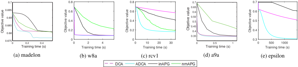
We reported in Table 1 the running time in second, the classification accuracy on test set and the sparsity (percentage of selected features) of solution . We also plot the curves of objective function values versus training time in Figure 1.
Concerning the classification accuracy, ADCA gives the best results for all 5 datasets (all four algorithms give the same result on madelon). As for the sparsity of solution, the four algorithms are comparable. All four algorithms give the same results on madelon and the best sparsity of solution on a9a is obtained by DCA, inAPG, nmAPG. nmAPG suppresses more features than the others on rcv1 while ADCA gives the best sparsity of solution on w8a,epsilon. In term of running time, ADCA is clearly the fastest one among the four compared algorithms. ADCA improve considerably the running time comparing to DCA: ADCA is up to 12.09 times faster than DCA (gisette). ADCA is faster than inAPG and nmAPG which also use acceleration technique. We can observe from Figure 1 that the objective functions of ADCA decrease drastically in few first iterations comparing to the others three algorithms.
Overall, among the four compared algorithms, ADCA is the fastest one while giving better classification accuracy and sparsity of solution.
5 Conclusion
We have rigorously studied ADCA, a variant of DCA with the aim of improving its performance. ADCA consists in incorporating the Nesterov's acceleration technique into DCA. We have proved that ADCA converges to a critical point of the standard DC program. Furthermore, we proved the convergence rate of ADCA under the Lojasiewics assumption. ADCA is then developed for the minimization of sum of two nonconvex functions problem, a special case of the standard DC program. Exploiting the fact that f(x) is differentiable with L-Lipschitz gradient, we propose, an efficient DC decomposition for which the corresponding ADCA scheme is inexpensive. To evaluate the performance of proposed algorithm, we consider the sparse binary logistic regression problem. ADCA for solving the latter is very inexpensive: it only required the soft thresholding operator which is explicitly computed. Numerical results showed that ADCA improves considerably the running time of DCA (up to 12.09 times faster than DCA) while giving similar or better classification accuracy and sparsity of solution. Furthermore, ADCA outperformed related accelerated proximal gradient methods such as non-monotone APG and inexact APG.
@inproceedings{ijcai2018p190,
  title     = {Accelerated Difference of Convex functions Algorithm and its Application to Sparse Binary Logistic Regression},
  author    = {Phan, Duy Nhat and Le, Hoai Minh and Le Thi, Hoai An},
  booktitle = {Proceedings of the Twenty-Seventh International Joint Conference on
               Artificial Intelligence, {IJCAI-18}},
  publisher = {International Joint Conferences on Artificial Intelligence Organization},
  editor    = {Jérôme Lang},
  pages     = {1369--1375},
  year      = {2018},
  month     = {7},
  note      = {Main track},
  doi       = {10.24963/ijcai.2018/190},
  url       = {https://doi.org/10.24963/ijcai.2018/190},
}
TY - CPAPER TI - Accelerated Difference of Convex functions Algorithm and its Application to Sparse Binary Logistic Regression AU - Phan, Duy Nhat AU - Le, Hoai Minh AU - Le Thi, Hoai An T2 - Proceedings of the Twenty-Seventh International Joint Conference on Artificial Intelligence, IJCAI-18 PB - International Joint Conferences on Artificial Intelligence Organization PY - 2018 SP - 1369 EP - 1375 DO - 10.24963/ijcai.2018/190 UR - https://doi.org/10.24963/ijcai.2018/190 ER -Copied
Machine-readable versions of this paper, for tools and AI agents:





