
Online Bridged Pruning for Real-Time Search with Arbitrary Lookaheads
Proceedings of the Twenty-Sixth International Joint Conference on Artificial Intelligence. Main track. Pages 510-516.
https://doi.org/10.24963/ijcai.2017/72
Keywords
- Planning and Scheduling: Real-time Planning
- Robotics and Vision: Motion and Path Planning
- Combinatorial & Heuristic Search: Heuristic Search
Abstract
Real-time search algorithms are relevant to time-sensitive decision-making domains such as video games and robotics. In such settings, the agent is required to decide on each action under a constant time bound, regardless of the search space size. Despite recent progress, poor-quality solutions can be produced mainly due to state re-visitation. Different techniques have been developed to reduce such a re-visitation with state pruning showing promise. In this paper, we propose a novel pruning approach applicable to the wide class of real-time search algorithms. Given a local search space of arbitrary size, our technique aggressively prunes away all states in its interior, possibly adding new edges to maintain the connectivity of the search space frontier. An experimental evaluation shows that our pruning often improves the performance of a base real-time search algorithm by over an order of magnitude.
This allows our implemented system to outperform state-of-the-art real-time search algorithms used in the evaluation.
- [Botea et al., 2004] A. Botea, M. Müller, and J. Schaeffer. Near Optimal Hierarchical Path-Finding. Journal of Game Development, 1(1):7-28, 2004.
- [Bulitko and Sampley, 2016] Vadim Bulitko and Alexander Sampley. Weighted lateral learning in real-time heuristic search. In Proceedings of the Symposium on Combinato- rial Search, 2016.
- [Bulitko et al., 2011] Vadim Bulitko, Yngvi Björnsson, Nathan Sturtevant, and Ramon Lawrence. Real-time Heuristic Search for Game Pathfinding. Applied Research in Artificial Intelligence for Computer Games. Springer, 2011.
- [Bulitko, 2016] Vadim Bulitko. Evolving real-time heuristic search algorithms. In Proceedings of the Fifteenth Inter- national Conference on the Synthesis and Simulation of Living Systems, 2016.
- [Geisberger et al., 2008] Robert Geisberger, Peter Sanders, Dominik Schultes, and Daniel Delling. Contraction Hier- archies: Faster and Simpler Hierarchical Routing in Road Networks. In Proceedings of the 7th International Confer- ence on Experimental Algorithms, WEA'08, pages 319- 333, 2008.
- [Hernández and Baier, 2012] Carlos Hernández and Jorge A. Baier. Avoiding and escaping depressions in real-time heuristic search. Journal of Artificial Intelligence Re- search, 43:523-570, 2012.
- [Koenig and Sun, 2009] Sven Koenig and Xiaoxun Sun. Comparing real-time and incremental heuristic search for real-time situated agents. Journal of Autonomous Agents and Multi-Agent Systems, 18(3):313-341, 2009.
- [Korf, 1990] R.E. Korf. Real-time heuristic search. Artificial Intelligence, 42(2-3):189-211, 1990.
- [Pochter et al., 2011] Nir Pochter, Aviv Zohar, and Jeffrey S Rosenschein. Exploiting problem symmetries in state- based planners. In Proceedings of the National Conference on Artificial Intelligence (AAAI), 2011.
- [Rivera et al., 2015] Nicolas Rivera, Jorge A. Baier, and Carlos Hernández. Incorporating weights into real-time heuristic search. Artificial Intelligence, 225:1-23, 2015.
- [Sharon et al., 2013] Guni Sharon, Nathan Sturtevant, and Ariel Felner. Online detection of dead states in real-time agent-centered search. In Sixth Annual Symposium on Combinatorial Search (SoCS), pages 167-174, 2013.
- [Sharon et al., 2014] Guni Sharon, Ariel Felner, and Nathan R. Sturtevant. Exponential deepening A* for real-time agent-centered search. In Proceedings of the Twenty-Eighth AAAI Conference on Artificial Intelligence, pages 871-877, 2014.
- [Shimbo and Ishida, 2003] Masashi Shimbo and Toru Ishida. Controlling the learning process of real-time heuristic search. Artificial Intelligence, 146(1):1-41, 2003.
- [Sturtevant and Bulitko, 2011] Nathan R. Sturtevant and Vadim Bulitko. Learning where you are going and from whence you came: H-and G-cost learning in real-time heuristic search. In Proceedings of the International Joint Conference on Artificial Intelligence, pages 365- 370, 2011. IJCAI
- [Sturtevant and Bulitko, 2016] Nathan Sturtevant and Vadim Bulitko. Scrubbing during learning in real-time heuristic search. Journal of Artificial Intelligence Research, 2016.
- [Sturtevant et al., 2010] N. R. Sturtevant, V. Bulitko, and Y. Björnsson. On learning in agent-centered search. In Proceedings of the Conference on Autonomous Agents and Multiagent Systems, pages 333-340, 2010.
- [Sturtevant et al., 2015] Nathan R. Sturtevant, Jason M. Traish, James R. Tulip, Tansel Uras, Sven Koenig, Ben Strasser, Adi Botea, Daniel Harabor, and Steve Rabin. The Grid-Based Path Planning Competition: 2014 Entries and Results. In Proceedings of the Eighth Annual Symposium on Combinatorial Search, SoCS, 2015.
- [Sturtevant, 2012] N. R. Sturtevant. Benchmarks for grid- based pathfinding. Transactions on Computational Intelli- gence and AI in Games, 4(2):144 -148, 2012.
- [Sturtevant, 2016] Nathan Sturtevant. Personal communica- tion. 2016.
- [Uras et al., 2013] Tansel Uras, Sven Koenig, and Carlos Hernández. Subgoal graphs for optimal pathfinding in eight-neighbor grids. In Proceedings of the Twenty- Third International Conference on Automated Planning and Scheduling, ICAPS, 2013.
References were extracted automatically from the PDF and may contain errors.
Full text extracted automatically from the PDF; figures, tables and equations may differ. The PDF is the version of record.
1 Introduction
Real-Time Heuristic Search (RTHS) [Korf, 1990] comprises a family of algorithms for solving deterministic search problems in time-constrained scenarios, where agents must act before a complete solution can be computed. It has applications in robotics and video games. To solve a search problem, RTHS algorithms (e.g., LSS-LRTA* [Koenig and Sun, 2009]) interleave planning and plan execution. On each iteration, most such algorithms build a bounded local-search space, select an action for execution and use learning mechanisms to update their heuristic function h. The learning updates make h more informed, eventually guaranteeing that the goal state will be reached.
In practical applications, such as video-game pathfinding, heuristic functions have local depressions and simple RTHS algorithms revisit some of the states many times [Shimbo and Ishida, 2003], resulting a phenomenon known as "scrubbing". This hampers the use of such algorithms in real-world applications [Bulitko et al., 2011]. While scrubbing is unavoidable in simple RTHS algorithms [Sturtevant and Bulitko,
2016], more complex techniques can mitigate or even eliminate scrubbing. These include actively avoiding heuristic depressions [Hern´andez and Baier, 2012], escaping depressions faster by accelerating the heuristic growth rate [Rivera et al., 2015; Bulitko and Sampley, 2016], and pruning states from the search space [Sharon et al., 2013].
We present a new approach to mitigating scrubbing and improving the resulting RTHS solution quality based on pruning. Our technique, PALMA (Pruning with Arbitrary Lookaheads and Macro Actions), is based on a simple idea: if in a local search the search frontier (the Open list) is a connected set of states, all states expanded in this search (the Closed list) can safely be pruned from the search space. If the frontier (Open list) is disconnected we still prune all states in Closed from the search space, but add new edges to ensure that states on the frontier remain reachable from each other.
A limited implementation of this idea was evaluated by Sharon et al. [2013] who detected and pruned at most a single expendable state per move. PALMA is more general and can prune much larger sets of states expanded during the search. In fact, by pruning all expanded states per move while adding new edges to preserve goal reachability, PALMA guarantees reaching the goal even without heuristic learning. Finally, PALMA can operate on top of any local-search-spacebuilding RTHS algorithm. Similarly to macro-edges used in previous route planning and pathfinding approaches, such as contraction hierarchies [Geisberger et al., 2008] for example, our new edges are shortcuts that allow avoiding intermediate nodes during a search.
We implement PALMA on top of LSS-LRTA* [Koenig and Sun, 2009] and call the resulting algorithm PALMA(LSSLRTA*). An empirical evaluation is performed on standard pathfinding benchmarks [Sturtevant, 2012]. We observe significant performance gains for a range of lookahead values. For lower lookahead values, the improvements on top of LSSLRTA* can exceed one order of magnitude. Even with deeper lookahead, the improvements remain significant. Overall, PALMA(LSS-LRTA*) outperforms high-performance RTHS algorithms used in our evaluation.
We formulate the real-time heuristic search problem in Section 2 and review related work in Section 3. We then discuss the idea of connectivity-preserving pruning in Section 4 and propose our novel method of implementing it in Section 5. This is followed by a theoretical analysis in Section 6 and an empirical evaluation in Section 7. A short discussion and future work directions conclude the paper.
2 ProblemFormulation
We use a standard formulation of the real-time heuristic search which we adopt from Bulitko [2016]. A search problem is a tuple (S,E, c, s0, sg, h), where S is a finite set of states (also called nodes), and E ⊂ S × S is a finite set of edges between them. S and E jointly define the search graph G which we assume to be undirected (i.e., (s, s′ ) ∈ E iff (s′ , s) ∈ E). A cost function c assigns a positive finite cost to each edge in E. Two states sa and sb are immediate neighbors iff there is an edge between them: (sa, sb) ∈ E; we denote the set of immediate neighbors of a state s by N(s). A path π in graph G = (S, E) is a sequence of states (s0, s1, . . . , sn) such that for all i ∈ {0, . . . , n - 1}, (si, si+1) ∈ E. If there exists a path starting with s and ending with t we say that t is reachable from s in G, denoted by s ❀G t. Given a graph (S,E) and a subset of nodes S′ in S, the graph induced by S′ is G′ = (S′ ,E′ ), where E′ = {(u, v) ∈ E | u, v ∈ S′ }. We assume that the search graph (S, E) is connected (i.e., any two vertices have a path between them) which makes it safely explorable. We also assume that the search graph is stationary (e.g., the edge weights do not change during search).
At all times t ∈ {0, 1, . . . } the agent occupies a single state st ∈ S, called the current state. The state s0 is the start state and is given as a part of the problem. The agent can change its current state, that is, move to any immediately neighboring state in N(s). The traversal incurs a travel cost of c(st, st+1). The agent solves the search problem at the earliest time it arrives at the goal state. The solution is a path P = (s0, . . . , sg). The cumulative cost of all edges in a solution is called the solution cost. The cost of the shortest possible path between states sa, sb ∈ S is denoted by h∗ (sa, sb). We abbreviate h∗ (s, sg) as h∗ (s). The suboptimality of the agent on a problem is the ratio of the solution cost the agent incurred to the cost of the shortest possible solution. Lower suboptimality values are preferred.
The agent has access to a heuristic h : S → [0,∞). The initial heuristic is a part of the problem specification and is meant to give the agent an estimate of the remaining cost to go. The search agent can modify the heuristic at will. We say that a search agent is real time iff the computation time between the agent's moves is upper-bounded by a constant independent of the number of states in the search space. A search algorithm is correct if its computed solutions (paths to goal) are valid, and complete if it outputs a solution to any search problem as defined above. With our pruning approach we aim to reduce the solution suboptimality and the total planning time while keeping the algorithm correct and complete.
For presentational clarity we introduce our pruning strategy on top of a commonly used LRTA*-style real-time search framework (Algorithm 1).
A search agent in this framework begins in the start state s0. It then executes a fixed loop until it reaches the goal sg (line 3). At each iteration∗ of the loop, the agent expands†
∗ Search performed within an iteration is called a search episode.
†A state is expanded if its immediate neighbors are generated.
input : search problem (S,E, c, s0, sg, h) output: solution path (s0, s1, . . . , sg) 1 t ← 0 2 ht ← h 3 while st ̸= sg do 4 form local search space Closed ∪ Open 5 set π to the shortest path connecting st and the most promising state in Open 6 update heuristic values in Closed 7 move the agent through every state in path π 8 t ← t + 1some states around its current state st (line 4). The expanded states comprise the Closed list. All states generated but not expanded constitute the Open list. Then the agent updates heuristic values of states in Closed (line 6). Finally, it moves from st to st+1, which is the most promising state in Open (line 7). The cycle then repeats until the goal state is reached. The goal state is never expanded. Thus, it can belong only to the Open list and is never removed from it.
3 RelatedWork
Pruning approaches mitigate the scrubbing problem of realtime heuristic search by permanently removing some states from the search graph. The graph is then reduced in size, decreasing the number of state revisits. The key questions are: how to efficiently identify the states to prune, how to preserve algorithm completeness and what impact on solution suboptimality the pruning will have.
Pochter et al. [2011] used graph automorphism to detect symmetries and reduce the search graph in planning. In realtime heuristic search, Sturtevant et al. [2010] identified two special types of states: dead-ends and redundant states. Informally, if a state is a dead-end then it cannot belong to an optimal path. Two or more states are redundant when only one of them is needed to preserve solution optimality. To identify such states, their algorithm, RIBS, learned the optimal g costs from the start state to a given state. Sturtevant and Bulitko [2011] adopted the pruning technique of RIBS and combined its g learning with the more traditional h learning. This has led to a stronger pruning performance.
Pruning techniques in RIBS and f-LRTA* rely on learning g and thus are not applicable to LRTA*-style algorithms, which learn h-values only. Sharon et al. [2013] introduced the notion of a locally expendable state as a state whose immediate neighbors are connected through themselves. Their algorithm then pruned away the agent's current state if it is found to be expendable. Note that their pruning technique was applied only to the local search space of a single state (i.e., lookahead of 1) and, in grid pathfinding, could create a checkerboard-like pattern of pruned states. Such a pattern would then preclude pruning other states as they become nonexpendable. Thus they pruned only the states whose heuristic was updated by the agent which, in the usual grid pathfinding, happens only around obstacles [Sturtevant, 2016].
By definition, the lookahead value is the the number of states expanded in one episode. With the lookahead of 1 only the current state is expanded.
Our pruning strategy is a generalization of their idea to arbitrarily large local search spaces and their frontiers. Furthermore, when the frontier of the local search space is disconnected, we still prune away the local search space and restore connectivity by adding new edges.
Contraction hierarchies (CHs) [Geisberger et al., 2008] introduce shortcut edges that can prune away intermediate nodes from a search. CHs have been used for optimal route planning on road maps and, more recently, for pathfinding on gridmaps [Sturtevant et al., 2015]. They are built in a preprocessing step. In fact, using macro-edges in gridmap pathfinding, as a way to avoid searching in a given area, is a popular idea in the literature (e.g., [Botea et al., 2004; Uras et al., 2013]). In contrast, our technique applies to realtime search, and it performs search-space contractions online.
4 Bridged Pruning
The main idea of our approach is to prune the search space of nodes that do not need to be considered as part of the search space in subsequent episodes. Pruning is performed after each search episode, right after the movement has concluded (i.e., immediately after line 7 in Algorithm 1).
Definition 1 (Pruning). Given a graph G = (S, E) and a set of states T ⊂ S, the result of pruning T from G is the graph induced from G by S \ T , denoted by G-T .
Definition 2 (Frontier). Given a graph G = (S, E) and a set of states T ⊂ S, the frontier of T , denoted by ∂GT (or simply by ∂T if G is clear from the context), is the set {s | (t, s) ∈ E, t ∈ T, s ̸∈ T}.
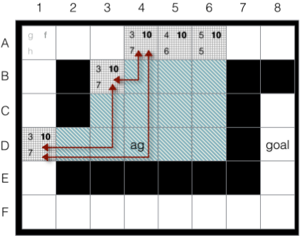
In undirected connected graphs, any set of nodes is connected. This property, however, may not hold true as a result of pruning states of T. Indeed, the frontier ∂T may become disconnected (this can be observed in Figure 2, described later, where ∂T are the gray dotted cells with three numbers each). A property that guarantees that the goal is reachable after pruning is that the frontier of the pruned area, ∂T , remains connected. Hence, we define the notion of bridged pruning, which accounts for the fact that, after generating G-T , extra edges can be added to G-T to connect (bridge) states in ∂T .
Definition 3 (Bridged Pruning). Given a graph G = (S, E) and a set of states T ⊂ S, the graph G⊖T is the result of a bridged pruning of T from G iff G⊖T is obtained from G-T by adding zero or more new edges between states in ∂GT such that ∂GT induces a connected subgraph of G⊖T .
Lemma 1 (Preserving Reachability). Let G⊖T be a bridged pruning of T from a graph G. Furthermore let s and t be such that s ❀G t. If s and t have not been pruned (i.e., are not in T) then s ❀G⊖T t.
Proof. Let π be a path inGfroms to t (depicted as the shorter trajectory in Figure 1). If π does not contain a state from T then π is a path between s and t in G⊖T and therefore s ❀G⊖T t. Otherwise, π is of the form π = (n1, . . . , nm), where n1 = s and nm = t. Since n1, nm ̸∈ T there is a non-empty subpath (ni, ni+1, . . . , nj) of states in T such that ni-1 and nj+1 are both in ∂T. As ∂T is connected in G⊖T , there must be another path between ni-1 and nj+1 in G⊖T (depicted as the dashed detour in the figure). Let σ denote its states from the second to the second-to-last. Since σ lies entirely in G⊖T , it has no states in T. Therefore the path π′ = (n1, . . . , ni-1, σ, nj+1, . . . , nm) contains at least one fewer state from T than π did. This process can be repeated until the constructed path has no states from T at all.
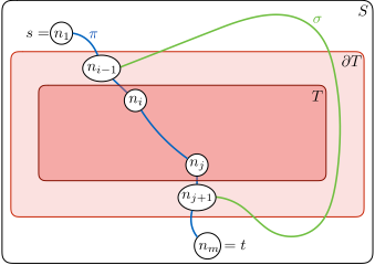
The important implication of Lemma 1 is that bridged pruning keeps the goal reachable from the agent's current state as long as neither the agent's current state nor the goal are pruned. We use this in the next section to show that our bridged-pruning system preserves the search completeness.
5 The PALMA PruningMethod
Above we have discussed bridged pruning, which ensures reachability of the goal state. We have not discussed yet how a bridged pruning can be carried out in practice. In this section we present PALMA, our implementation of bridged pruning. While PALMA can be used in any undirected graph, we will use grid pathfinding to illustrate it.
The four-connected grid in Figure 2 will serve as a running example to describe PALMA. Black cells are obstacles, whereas all other cells form the traversable area. Cell D8 is
Algorithm 2: PALMA
input : a set of states Closed, a search weighted graph G = (S, E, c) output: G⊖Closed 1 S′ ←S \ Closed 2 E′ ←E ∩ (S′ ×S′ ) 3 Enew, cnew ← PALMACONNECT(∂Closed,G) 4 E′ ←E′ ∪Enew 5 c′ ← c ∪ cnew 6 return G′ = (S′ ,E′ , c′ )the goal. D4 is the agent location at the beginning of the iteration. The figure shows a local search space formed in line 4 of Algorithm 1. In this example we used an A*-shaped local search. Dotted cells comprise the Open list. They are labeled with h, g and f = g+h (clockwise from the bottom left). Diagonally striped cells form the Closed list. After the search, the agent follows a path to a lowest f-value state in the Open. In our example, all states in the Open have f = 10 so any of them can be the state to go to, depending on the tie-breaking schema employed.
After line 7 of Algorithm 1, we invoke our bridged pruning procedure PALMA. Algorithm 2 gives an overview of PALMA. Its input is the current search graph and the Closed list which contains a set of states expanded in the current search episode. In the first two lines, G-Closed is computed. Then additional edges Enew are computed by calling PALMACONNECT in line 3. That function returns weighted edges that reconnect the frontier ∂Closed if ∂Closed becomes disconnected and returns an empty set otherwise. The function PALMA then returns G⊖Closed, the result of the bridged pruning of Closed from G (line 6). The current search graph is replaced with the graph returned by PALMA.
We will now walk through PALMACONNECT, presented as Algorithm 3. PALMACONNECT adds new edges to make sure that the frontier is connected. Specifically, in line 5 we check whether the graph GB, the graph induced by ∂Closed (line 3), is connected. If so there is no need to add any new edges because there already exists a path between any two states of ∂Closed that visits only states in ∂Closed. If GB is not connected, however, we compute an edge between two states that lie in two different disconnected components of GB in line 9. The cost assigned to an action connecting two states u and v is the cost of a shortest path between u and v in the search graph before pruning away the states in Closed at the current episode (lines 10 and 11).
Algorithm 3 specifies neither how to select states in the connected components in line 8 nor how to compute the cost of new edges in line 10. In this paper we used the following implementation. For each of the r connected components Gi; i ∈ {1, . . . , r} we select the state si = argmin{g(s)|s ∈ Gi}. To compute the costs of the new edges (si, sj); i, j ∈ {1, . . . , r}, we run r - 1 Dijkstra searches starting them in s1, s2, . . . , sr-1 respectively. A Dijkstra search is restricted to GL, is started in si and is stopped as soon as optimal costs from si to all states sj, j > i are computed. This process ensures that a path will be discovered for every pair of selected
Algorithm 3: PALMACONNECT
input : a set of states, Closed, a weighted graph G output: a set of new weighted edges between states in Closed 1 Enew ← ∅ 2 cnew ← ∅ 3 GB ← subgraph of G induced by ∂Closed 4 GL ← subgraph of G induced by Closed ∪ ∂Closed 5 if GB is not connected then 6 {G1, . . . , Gr} ← connected components of GB 7 for each pair (i, j) such that 1 ≤ i < j ≤ r do 8 select a state si in Gi and a state sj in Gj 9 Enew ← Enew ∪ {(si, sj ), (sj , si)} 10 c′ ← cost of a shortest path between si and sj in GL 11 cnew ← cnew ∪ {((si, sj ), c′ ), ((sj , si), c′ )} 12 return Enew, cnewstates while bounding the search effort.‡
To illustrate the process of adding new edges, we revisit the example in Figure 2. Recall that the dotted cells with three numbers each compose the Open list. The Open list has three connected components: {D1}, {B3} and {A4,A5,A6}. Two of the three connected components have one state each ({D1} and {B3}). For the three-state component {A4, A5, A6} the state selected for connection is A4. We then compute shortest paths between D1 and B3; B3 and A4; and D1 and A4. For each such path we add a single new weighted edge (e.g., (D1,B3) will have a cost of 4). New edges are shown as bi-directional arrows in the figure. All diagonally striped states (the Closed list) are then pruned out from the search graph G.
Note that the modifications to the search graph made by bridged pruning exist solely in the agent's representation of the world. The actual graph traversed by the agent remains unchanged throughout the search. So when PALMA prunes a state, it simply marks it as such in the agent's representation of the world. When PALMA adds a new edge, it actually remembers a sequence of states in the original graph the agent would have to travel in the world to traverse the new edge. In our running example, traversing the new edge between states B3 and D1 would make the agent visit the states C3, D3, and D2, marked as "pruned" from the search graph.
6 Theoretical Analysis
We will now discuss the completeness of RTHS algorithms equipped with PALMA. Let PALMA(A) be an application of PALMA to a real-time heuristic algorithm A which itself conforms to the framework presented in Algorithm 1.
Lemma 2. PALMA(A) runs at most n - 1 search episodes.
Proof. After each search episode, at least one state is pruned from the search graph by PALMA. Unless the goal is reached earlier, after n - 2 episodes the remaining search graph will contain at most 2 states. Thus, the goal state will be generated within the next search episode which will lead to the agent's reaching the goal on the next episode.
‡We evaluated two other ways of selecting a representative state si from each connected component Gi: (i) minimizing f(si) instead of g(si) and (ii) minimizing c′ (si, sj) across all i, j. Both proved inferior in the experiments we ran.
In real-time heuristic search, heuristic updates are often used to ensure completeness. Without such updates, algorithms such as LRTA* can degenerate to simple hill-climbing and get forever stuck in a local heuristic depression. Remarkably, the bridged pruning implemented in PALMA guarantees completeness on its own, without any heuristic learning.
Lemma 3. When using PALMA(A), the goal is always reachable from the agent's current state.
Proof. The agent's current state is never pruned as the agent moves to Open before pruning the Closed list. The goal is never pruned as it can never be in Closed. It follows from Lemma 1 that the goal is reachable from every state in the bridge-pruned search space, including the agent's state.
Theorem 1. For any RTHS algorithm A that fits the framework in Algorithm 1, PALMA(A) is correct (i.e., terminates only at the goal state) and complete (i.e., reaches the goal state) regardless of any learning (or lack thereof) of the heuristic function.
Proof. After each search episode, the goal remains reachable from the agent's position, according to Lemma 3 and therefore PALMA(A) terminates only when A terminates. A terminates only upon reaching the goal (line 3 in Algorithm 1). Thus PALMA(A) is correct. PALMA(A) is complete as it terminates after at most n-1 search episodes by Lemma 2.
For simplicity, our analysis focused on solvable problems. With minor modifications to Algorithm 3, on a finite graph PALMA(A) can detect that no solution exists (i.e., the goal is not reachable from the agent's initial state). We omit the proof due to space limitations. Being able to detect that a solution does not exist is a benefit PALMA brings to LRTA*- style algorithms that cannot do so by themselves.
7 Empirical Evaluation
PALMA is applicable to any real-time search algorithm that conforms to Algorithm 1. For our evaluation, we chose to apply it on top of LSS-LRTA* [Koenig and Sun, 2009], which is a high-performance commonly used real-time search algorithm generalizing the classic LRTA* algorithm [Korf, 1990]. To assess the resulting algorithm performance relative to the state of the art we compare it to wLSS-LRTA* [Hern´andez and Baier, 2012] and EDA* [Sharon et al., 2014]. The former is a representative of the depression-avoiding family of algorithms while the latter is an IDA*-inspired algorithm that does not fit into the framework of Algorithm 1 but was shown to have good performance with respect to depression-avoiding algorithms [Sharon et al., 2014]. For both algorithms we use the best parameters as reported in the original publications (w = 8 for wLSS-LRTA* and C = 8 for EDA*).
We implemented all algorithms in C over a common code base. For LSS-LRTA* and its variants, we use a binary heap for Open in which ties are broken in favor of larger g-values.
We took maps from the commonly used MovingAI pathfinding repository [Sturtevant, 2012]. We used all five 1024×1024 StarCraft maps, 30 maze maps of size 512×512 (corridor widths of 4, 8, 16), all 512×512 maps World of Warcraft III (WC3) and all roommaps of size 512×512. Finally, as a fifth benchmark, we consider the same maze maps, but with 1% of their obstacles removed. For each map we generated 100 random solvable problems. Each map is modeled as an undirected eight-connected grid, with costs set to 1 for cardinal moves and √2 for diagonal moves. The octile distance is used as a heuristic. Experiments are run on a 2.60GHz Intel Core i7 machine under Linux, as a single-threaded process.
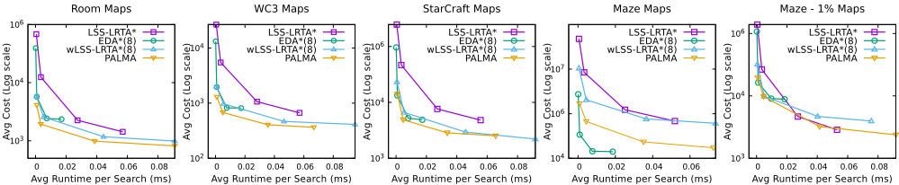
By varying the lookahead value (i.e., number of expanded states per episode) LSS (1, 10, 100 and 200) we can trade solution quality with the time per search episode as shown in Figure 3. When the time spent per each search is relatively uniform between episodes, as is the case with all of these algorithms, these plots provide a fair comparison between algorithms. They show PALMA(LSS-LRTA*) is the bestperforming algorithm in four out of five benchmarks. In the remaining domain (mazes), for all but the smallest lookahead value, EDA* computes shorter solutions in a shorter time.
Table 1 shows the average solution cost, the average perproblem runtime, and the average number of search episodes. Best performance per lookahead value is shown in bold. Given a combination c of a lookahead value and a map type (i.e., a block in the table), we say that that algorithm dominates the others for combination c if it has both the lowest solution cost and the lowest runtime. PALMA(LSS-LRTA*) is the dominant algorithm in 15 out of 20 combinations (blocks in the table). EDA* dominates in three out of 20 combinations, all corresponding to mazes. In two out of the 20 combinations no algorithm is dominant yet PALMA(LSS-LRTA*) has the shortest solution in one of these two combinations.
Comparing PALMA(LSS-LRTA*) to its base algorithm LSS-LRTA*, Table 1 shows that PALMA(LSS-LRTA*) dominates LSS-LRTA* in all 20 combinations. PALMA's improvements can reach a factor of 20 in terms of both solution cost and runtime. Overall PALMA(LSS-LRTA*) shows significant performance improvements over state-of-the-art algorithms used in our evaluation. PALMA(LSS-LRTA*) consistently requires the smallest number of search episodes.
| WC3 Maps | SC Maps | Mazes | Mazes - 1%obst. | |||||||||||||
|---|---|---|---|---|---|---|---|---|---|---|---|---|---|---|---|---|
| LSS-LRTA* EDA*(8) | LSS 1 | Cost 68,478 | Room Maps Time 31.25 4.55 | Epis. 63,574 35,905 | Cost 26,624 13,212 | Time 12.50 1.52 | Epis. 24,723 11,725 | Cost 246,763 96,103 | Time 116.98 11.47 | Epis. 229,262 85,986 | Cost 4,774,362 273,001 1,049,026 | Time 2,103.83 33.22 | Epis. 4,470,766 257,987 | Cost 139,137 107,600 | Time 63.17 15.38 | Epis. 128,661 99,268 |
| wLSS-LRTA(8) | 1 1 | 39,330 5,843 | 3.03 | 5,386 | 1,995 | 1.10 | 1,808 | 23,262 | 12.09 | 20,598 | 466.29 | 891,429 | 32,154 | 16.36 | 28,494 | |
| PALMA | 1 | 4,113 | 2.66 | 3,142 | 1,299 | 0.92 | 973 | 14,048 | 8.34 | 9,292 | 168,440 | 70.73 | 86,666 | 19,488 | 11.08 | 13,104 |
| LSS-LRTA* | 10 | 12,432 | 18.90 | 5,439 | 5,459 | 8.32 | 2,352 | 46,477 | 72.02 | 20,468 | 846,310 | 1,211.58 | 365,178 | 26,496 | 38.72 | 11,169 |
| EDA*(8) | 10 | 5,728 | 2.86 | 3,591 | 1,960 | 0.97 | 1,173 | 13,302 | 7.44 | 8,599 | 33,925 | 22.46 | 25,799 | 16,330 | 10.66 | 9,927 |
| wLSS-LRTA(8) | 10 | 2,565 | 2.99 | 571 | 974 | 1.12 | 207 | 6,632 | 7.74 | 1,447 | 204,548 | 187.95 | 42,401 | 9,883 | 10.93 | 2,200 |
| PALMA | 10 | 1,936 | 2.02 | 424 | 678 | 0.68 | 135 | 4,882 | 4.85 | 1,034 | 66,810 | 40.93 | 9,339 | 9,775 | 8.56 | 1,848 |
| LSS-LRTA* | 100 | 2,251 | 7.66 | 279 | 1,064 | 3.52 | 125 | 7,624 | 26.90 | 989 | 122,731 | 375.08 | 14,903 | 4,662 | 14.17 | 520 |
| EDA*(8) | 100 | 2,424 | 2.63 | 360 | 822 | 0.89 | 118 | 5,224 | 6.85 | 860 | 14,351 | 19.84 | 2,580 | 9,041 | 9.59 | 993 |
| wLSS-LRTA(8) | 100 | 1,174 | 3.35 | 75 | 466 | 1.21 | 26 | 2,939 | 8.75 | 191 | 76,335 | 174.37 | 4,769 | 4,687 | 11.66 | 290 |
| PALMA | 100 | 987 | 2.34 | 58 | 405 | 0.71 | 20 | 2,853 | 5.82 | 173 | 23,273 | 30.52 | 870 | 3,223 | 6.37 | 153 |
| LSS-LRTA* | 200 | 1,427 | 6.52 | 114 | 667 | 2.78 | 49 | 4,816 | 23.10 | 415 | 68,297 | 277.87 | 5,356 | 2,865 | 10.64 | 201 |
| EDA*(8) | 200 | 2,351 | 3.25 | 188 | 812 | 1.09 | 63 | 4,881 | 7.73 | 448 | 14,110 | 24.43 | 1,316 | 8,860 | 9.19 | 497 |
| wLSS-LRTA(8) | 200 | 989 | 4.04 | 44 | 411 | 1.47 | 16 | 2,214 | 9.05 | 99 | 60,897 | 188.86 | 2,564 | 3,959 | 12.35 | 164 |
| PALMA | 200 | 816 | 2.96 | 32 | 365 | 0.79 | 12 | 2,522 | 6.43 | 98 | 17,210 | 29.58 | 408 | 2,375 | 6.92 | 75 |
| LSS | r | Avg # Succ | Max # Succ | |
|---|---|---|---|---|
| Room maps | 1 | 1.41 | 4.9 | 8.3 |
| 10 | 1.67 | 5.9 | 8.3 | |
| 100 | 3.21 | 6.9 | 9.7 | |
| 200 | 4.45 | 7.1 | 11.4 | |
| 1 | 1.19 | 5.8 | 8.1 | |
| WC3 10 | 1.16 | 6.6 | 8.1 | |
| maps 100 | 1.04 | 7.3 | 8.1 | |
| 200 | 1.07 | 7.4 | 8.1 | |
| 1 | 1.36 | 5.1 | 8.9 | |
| SC 10 | 1.40 | 6.1 | 8.5 | |
| maps 100 | 1.57 | 7.1 | 8.5 | |
| 200 | 1.76 | 7.3 | 8.7 | |
| 1 | 1.57 | 4.3 | 9.6 | |
| Maze 10 | 1.71 | 5.5 | 10.2 | |
| maps 100 | 2.23 | 6.7 | 9.4 | |
| 200 | 2.62 | 6.8 | 9.9 | |
| 1 | 1.51 | 4.5 | 8.7 | |
| Maze-1% maps | 10 | 1.66 | 5.6 | 9.2 |
| 100 | 2.51 | 6.7 | 9.7 | |
| 200 | 3.22 | 6.9 | 10.5 |
PALMA dynamically removes and adds edges to the search graph, varying the number of successors that a node can have and therefore its expansion time. Furthermore, the time effort required to add new edges depends on the size of the Open list (to check if the list is connected) and the number r of connected components of the Open list (as we run r - 1 Dijkstra searches to add edges between connected components). Table 2 shows summary statistics relevant to these computations. First it shows the average number of connected components (r) which turns out to be small, ranging from 1.04 to 4.45. In 13 out of the 20 combinations, the average r is below 2 implying that often the Open list is already connected and no Dijkstra searches are needed at all.
As PALMA adds new edges, we inspected the branching factor of the pruned graph (i.e., the number of successors for a state). Table 2 reports the average and the maximum number of state successors. Without new edges, an eight-connected grid map has at most 8 successors for any state. PALMA does not increase it substantially, with the maximum values ranging from 8.1 to 11.4. In 11 out of the 20 combinations, the maximum number of successors does not exceed 9.
8 Conclusion
Real-time heuristic search algorithms often produce lowquality solutions due to state re-visitation. Pruning states from the graph has shown promise in previous work but was limited to the basic case of removing the current state.
We presented a principled approach to pruning arbitrarily large sets of states while preserving the underlying algorithm's correctness and completeness. Our pruning can be implemented on top of most real-time search algorithms. Its aggressive pruning guarantees completeness on its own, without relying on heuristic learning. An empirical evaluation against state-of-the-art algorithms shows significant benefits.
Future work will investigate how pruning from a problem instance can be re-used in solving another problem instance. We also plan to perform an evaluation on scenarios with partial terrain knowledge.
Acknowledgements
Carlos Hern´andez and Jorge Baier were partly funded by Fondecyt grants 1150328 and 1161526.
@inproceedings{ijcai2017p72,
  title     = {Online Bridged Pruning for Real-Time Search with Arbitrary Lookaheads},
  author    = {Hernandez, Carlos and Botea, Adi and Baier, Jorge A. and Bulitko, Vadim},
  booktitle = {Proceedings of the Twenty-Sixth International Joint Conference on
               Artificial Intelligence, {IJCAI-17}},
  publisher = {International Joint Conferences on Artificial Intelligence Organization},
  editor    = {Carles Sierra},
  pages     = {510--516},
  year      = {2017},
  month     = {8},
  note      = {Main track},
  doi       = {10.24963/ijcai.2017/72},
  url       = {https://doi.org/10.24963/ijcai.2017/72},
}
TY - CPAPER TI - Online Bridged Pruning for Real-Time Search with Arbitrary Lookaheads AU - Hernandez, Carlos AU - Botea, Adi AU - Baier, Jorge A. AU - Bulitko, Vadim T2 - Proceedings of the Twenty-Sixth International Joint Conference on Artificial Intelligence, IJCAI-17 PB - International Joint Conferences on Artificial Intelligence Organization PY - 2017 SP - 510 EP - 516 DO - 10.24963/ijcai.2017/72 UR - https://doi.org/10.24963/ijcai.2017/72 ER -Copied
Machine-readable versions of this paper, for tools and AI agents:





