
Lossy Compression of Pattern Databases Using Acyclic Random Hypergraphs
Proceedings of the Twenty-Sixth International Joint Conference on Artificial Intelligence. Main track. Pages 4376-4383.
https://doi.org/10.24963/ijcai.2017/611
Keywords
- Combinatorial & Heuristic Search: Heuristic Search
- Planning and Scheduling: Search in Planning and Scheduling
Abstract
A domain-independent heuristic function created by an abstraction is usually implemented using a Pattern Database (PDB), which is a lookup table of (abstract state, heuristic value) pairs. PDBs containing high quality heuristic values generally require substantial memory space and therefore need to be compressed. In this paper, we introduce Acyclic Random Hypergraph Compression (ARHC), a domain-independent approach to compressing PDBs using acyclic random r-partite r-uniform hypergraphs. The ARHC algorithm, which comes in Base and Extended versions, provides fast lookup and a high compression rate. ARHC-Extended achieves higher quality heuristics than ARHC-Base by decreasing the heuristic information loss at the cost of some decrease in the compression rate. ARHC shows higher performance than level-by-level Bloom filter PDB compression in all experiments conducted so far.
- [Anderson et al., 2007] Kenneth Anderson, Robert Holte, and Jonathan Schaeffer. Partial pattern databases. In Pro- ceedings of the Seventh International Symposium on Ab- straction, Reformulation, and Approximation, pages 20- 34, 2007.
- [Bloom, 1970] Burton H. Bloom. Space/time trade-offs in hash coding with allowable errors. Communications of the ACM, 13(7):422-426, 1970.
- [Botelho et al., 2007] Fabiano C. Botelho, Rasmus Pagh, and Nivio Ziviani. Simple and space-efficient minimal perfect hash functions. In Proceedings of the Tenth In- ternational Workshop on Data Structures and Algorithms, volume 4619 of Lecture Notes in Computer Science, pages 139-150. Springer, 2007.
- [Breyer and Korf, 2010] Teresa Maria Breyer and Richard E. Korf. 1.6-bit pattern databases. In Proceedings of the Twenty-Fourth AAAI Conference on Artificial Intelligence, Atlanta, Georgia, USA, July 11-15, 2010.
- [Culberson and Schaeffer, 1998] Joseph Culberson and Jonathan Schaeffer. Pattern databases. Computational Intelligence, 14(3):318-334, 1998.
- [Czech et al., 1997] Zbigniew J. Czech, George Havas, and Bohdan S. Majewski. Perfect hashing. Theoretical Com- puter Science, 182(1-2):1 -143, 1997.
- [Edelkamp and Kissmann, 2008] Stefan Edelkamp and Peter Kissmann. Partial symbolic pattern databases for optimal sequential planning. In KI 2008: Advances in Artificial Intelligence, 31st Annual German Conference on AI, KI 2008, Kaiserslautern, Germany, September 23-26, 2008. Proceedings, pages 193-200, 2008.
- [Edelkamp, 2001] Stefan Edelkamp. Planning with pattern databases. In Proceedings of the Sixth European Confer- ence on Planning, pages 13-24, 2001.
- [Edelkamp, 2002] Stefan Edelkamp. Symbolifc pattern databases in heuristic search planning. In Proceedings of the Sixth International Conference on Artificial Intel- ligence Planning Systems, April 23-27, 2002, Toulouse, France, pages 274-283, 2002.
- [Felner et al., 2007] Ariel Felner, Richard E. Korf, Ram Meshulam, and Robert C. Holte. Compressed pattern databases. Journal of Artificial Intelligence Research, 30:213-247, 2007.
- [Hart et al., 1968] Peter E. Hart, Nils J. Nilsson, and Bertram Raphael. A formal basis for the heuristic determination of minimum cost paths. IEEE Transactions on Systems Science and Cybernetics, SSC-4(2):100-107, 1968.
- [Helmert and Lasinger, 2010] Malte Helmert and Hauke Lasinger. The Scanalyzer domain: Greenhouse logistics as a planning problem. In Proceedings of the Twentieth Inter- national Conference on Automated Planning and Schedul- ing, pages 234-237, 2010.
- [Holte et al., 2014] Robert Holte, Broderick Arneson, and Neil Burch. PSVN manual (june 20, 2014). Technical Re- port 14-03, Department of Computing Science, University of Alberta, 2014.
- [Jensen et al., 2002] Rune M. Jensen, Randal E. Bryant, and Manuela M. Veloso. SetA*: An efficient BDD-based heuristic search algorithm. In Proceedings of the Eigh- teenth National Conference on Artificial Intelligence and Fourteenth Conference on Innovative Applications of Arti- ficial Intelligence, pages 668-673, 2002.
- [Korf, 1985] Richard. E. Korf. Depth-first iterative- deepening: An optimal admissible tree search. Artificial Intelligence, 27(1):97-109, 1985.
- [Majewski et al., 1996] Bohdan S. Majewski, Nicholas C. Wormald, George Havas, and Zbigniew J. Czech. A family of perfect hashing methods. Computer Journal, 39(6):547-554, 1996.
- [Mitzenmacher and Upfal, 2005] Michael Mitzenmacher and Eli Upfal. Probability and Computing: Randomized Algorithms and Probabilistic Analysis. Cambridge University Press, 2005.
- [Sadeqi and Hamilton, 2016] Mehdi Sadeqi and Howard J. Hamilton. Efficient representation of pattern databases using acyclic random hypergraphs. In Proceedings of the Twenty-Sixth International Conference on Automated Planning and Scheduling, London, UK, June 12-17, pages 258-266, 2016.
- [Samadi et al., 2008] Mehdi Samadi, Maryam Siabani, Ariel Felner, and Robert Holte. Compressing pattern databases with learning. In Proceedings of the Eighteenth Euro- pean Conference on Artificial Intelligence, pages 495-499, 2008.
- [Sturtevant et al., 2014] Nathan R. Sturtevant, Ariel Felner, and Malte Helmert. Exploiting the Rubik's cube 12-edge PDB by combining partial pattern databases and Bloom filters. In Proceedings of the Seventh Annual Symposium on Combinatorial Search, 2014.
- [Zobrist, 1970] Albert L. Zobrist. A new hashing method with application for game playing. Technical Report 88, 1970.
References were extracted automatically from the PDF and may contain errors.
Full text extracted automatically from the PDF; figures, tables and equations may differ. The PDF is the version of record.
1 Introduction
A heuristic function is used by search algorithms such as A* [Hart et al., 1968] and IDA* [Korf, 1985] to prioritize their node expansion. An admissible heuristic function never overestimates the cost of reaching the goal state from any given state and guarantees that A* and IDA* will find optimal solutions [Hart et al., 1968; Korf, 1985]. Admissible heuristic functions can be created effectively using abstraction and are usually stored in memory in an efficient lookup table of (abstract state, heuristic value) pairs called a pattern database (PDB) [Culberson and Schaeffer, 1998]. Typically, larger PDBs contain more accurate heuristic values. Unfortunately, even with efficient representations, PDBs may not fit in memory. A common technique to address this problem is to compress the PDB.
Several approaches are proposed in the literature for compression of PDBs. One approach is min compression [Felner et al., 2007], which divides a PDB into buckets of size k and stores only the minimum value in each bucket. Storing the minimum value guarantees the admissibility of heuristic values in the compressed PDB. PDB compression can also be achieved by using a Partial Pattern Database (PPDB) [Anderson et al., 2007] in which only heuristic values up to and including a certain maximum value (here called v) are stored in the compressed PDB and a value v + 1 is used for the remaining abstract states. A recent paper by Sturtevant et al. [2014] illustrates that PPDBs that are effectively implemented by Bloom filters can perform better than min compression. Specifically, one particular variation of Bloom filter PPDBs for an abstraction of Rubik's cube shows superior performance over min compression.
We introduce the Acyclic Random Hypergraph Compression (ARHC) algorithm for compressing PDBs. It provides fast lookup and a high compression rate. We begin by explaining the role of abstraction in creating domainindependent heuristics represented using PDBs and existing techniques for compressing them. We then describe the ARHC algorithm for compressing PDBs using acyclic random hypergraphs. This algorithm can be considered to be an extension of the PDB representation approach introduced by Sadeqi and Hamilton [2016]. We describe two versions of ARHC: ARHC-Base provides higher compression and lower heuristic quality and ARHC-Extended provides higher heuristic quality at the expense of some decrease in the compression rate. We then show the effectiveness of ARHC by comparing it to a level-by-level Bloom filter PPDB [Sturtevant et al., 2014], in which each level of the PPDB is represented by a Bloom filter.
The experimental results show that ARHC performs substantially better than a level-by-level Bloom filter PPDB with respect to three measures. The main advantages of ARHC are its effectiveness with respect to the space usage and lookup speed and its independence of the problem domain and abstraction of interest.
2 Abstractions, PDBs, and PDB Compression
Domain-independent heuristics for a problem formulated as a state space search can be derived effectively using abstraction. To do so, we use abstraction to transform the original search problem into a simplified version called the abstract problem. The abstract problem is solved and the solution in the abstract space is used as a heuristic. More precisely, distances in the abstract state space can be used as heuristic values when solving the original problem. A pattern database is constructed by comprehensive expansion of the abstract state space, which is usually accomplished by performing a breadth first search starting from the abstract goal state and moving backwards in the abstract space. For each abstract state, its corresponding distance to the abstract goal state is stored in the PDB. This PDB is consulted by the search algorithms to obtain heuristic values efficiently.
Two types of compression are applied to PDBs: lossless, where all heuristic values in the original PDB are retained, and lossy, where heuristic values in the compressed PDB are less than or equal to their corresponding values in the original PDB (to guarantee admissibility).
In a lossless compression, PDB memory usage is decreased while retaining the total heuristic information in the original PDB. Lossless compression is not always effective because of the limitations of existing approaches or simply because even after substantial compression, the compressed PDB does not fit in memory. Binary Decision Diagrams (BDDs) [Edelkamp, 2002; Jensen et al., 2002], 1.6-bit pattern databases [Breyer and Korf, 2010] and ARH [Sadeqi and Hamilton, 2016] are among the most effective approaches for lossless compression of PDBs.
In lossy compression, some heuristic information present in the original PDB is allowed to be lost but all heuristic values must remain admissible. An effective lossy compression scheme tries to minimize the loss of heuristic information while maintaining admissibility.
A simple approach for lossy compression of PDBs is min compression [Felner et al., 2007], in which a PDB with N entries is divided into buckets of size k and only the minimum heuristic value in each bucket is stored. Storing the minimum value in each bucket guarantees admissibility. When nearby entries in the PDB have similar heuristic values, grouping them in buckets causes little information loss. This, for example, happens when the abstract states that form a clique (all adjacent to each other in the abstract space) are entries close to each other in the PDB. Due to such groupings, min compression is effective in some problem domains, such as 4-peg Towers of Hanoi [Felner et al., 2007].
Samadi et al. [2008] proposed learning heuristic values using an Artificial Neural Network (ANN). They also used a lookup table where they placed an admissible value for every case where the ANN predicted an inadmissible value. When looking up a heuristic value corresponding to an abstract state, this table is first consulted. If the abstract state is in the table, the heuristic value is returned immediately. Otherwise, the ANN is used to calculate the heuristic value.
PPDBs [Anderson et al., 2007] are another important technique for lossy compression of PDBs. A PPDB that only stores up to and including a certain depth v of a given PDB is usually denoted PPDBv (depth is equivalent to distance from the goal). PPDBs can be effectively implemented using a partial symbolic PDB [Edelkamp and Kissmann, 2008]. Bloom filters have also proven to be effective for PPDB implementation [Sturtevant et al., 2014].
3 Acyclic RandomHypergraph PDBs
An efficient representation of PDBs using acyclic random hypergraphs was proposed by Sadeqi and Hamilton [2016]. The basic idea of the ARH approach is to populate a lookup table in such a way that the heuristic value associated with an abstract state can be obtained from the combination of three values in this table. These three values are at table positions determined by the three hash values of the abstract state. Each entry in the lookup table corresponds to a vertex in an acyclic random r-partite r-uniform hypergraph generated by the ARH procedure and the three different entries calculated using the three hash functions, correspond to a hyperedge in this hypergraph. The aforementioned lookup table is produced by a two-step procedure. First, an acyclic random rpartite r-uniform hypergraph is generated by a process called mapping. The vertices of this hypergraph, which correspond to the lookup table entries, are then assigned appropriate values in the assigning step. These steps are described below.
3.1 Step 1: Mapping
A hypergraph G is a generalization of a conventional undirected graph where each edge has a size of two or more, i.e., it connects two or more vertices. If all the edges in G are of size r, then G is an r-uniform hypergraph or r-graph for short. An r-partite r-uniform hypergraph Gr = (V,E) has a vertex set V = ∪r-1 i=0 Vi where ∀i, j, i ̸= j : Vi ∩ Vj = ∅ and each edge has only one vertex from each Vi, i.e., no edge has two or more vertices from the same Vi. In a random r-partite r-uniform hypergraph Gr = (V,E), each edge in E is generated by randomly choosing one from all possible edges with repetitions allowed.
The goal of the mapping step is to find a random r-partite r-uniform hypergraph that has no cycles. Here we consider a hypergraph to be acyclic if and only if some sequence of repeated deletions of edges containing at least one vertex of degree 1 yields a hypergraph with no edges [Czech et al., 1997]. In the mapping step, we repeatedly generate random r-partite r-uniform hypergraphs until we find an acyclic one. If certain conditions are met, we are guaranteed to find an acyclic random r-partite r-uniform hypergraph with high probability: for a graph Gr = (V,E), the space of random r-partite r-uniform hypergraphs is dominated by acyclic ones when |V | ≥ cr|E|. cr = c(r) is a constant and has a minimum of approximately 1.23 at r = 3 [Czech et al., 1997], i.e., the smallest acyclic random r-partite r-uniform hypergraphs are 3-graphs.
An algorithm suggested by Majewski et al. [1996] is used to detect whether a hypergraph Gr has any cycles. It starts by queuing every edge of hypergraph Gr that has at least one vertex with degree one. The edges in this queue are then dequeued one by one, removed from the hypergraph Gr, and stored in a list L, for later use in step 2. After removing an edge from the hypergraph, if any of its vertices has degree one now, the edge that contains that vertex is enqueued in the queue. This is repeated until the queue is empty. Gr is acyclic if all its edges are removed by the algorithm.
3.2 Step 2: Assigning
After finding an acyclic random r-partite r-uniform hypergraph Gr in the mapping step, the appropriate values are assigned to the vertices of this hypergraph in the manner similar to what is proposed by Botelho et al. [2007]. The vertices of hypergraph Gr correspond to the entries of the lookup table T. We start by initializing all the entries in T to 0. We then move backwards in the list of edges L created in the mapping step. By traversing L backwards, we never encounter an edge such that all its vertices have already been assigned values (see [Sadeqi and Hamilton, 2016] for more details). For every edge e dequeued from this list from tail to head, we set the value for its unassigned vertices such that the summation of values of these vertices modulo the number of distinct entry values in the PDB is equal to the heuristic value of the abstract state corresponding to edge e in the hypergraph.
3.3 The ARHCApproach: Acyclic Random Hypergraph PPDBs for Lossy Compression
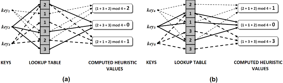
We propose ARHC, a PDB compression algorithm based on the idea of acyclic random hypergraph PDBs. Ideally, we would like to implement a PPDBv that retains heuristic values 0 to v and dedicates value v + 1 to the abstract states with heuristic values greater than v. We say such a PPDB is perfect. As an example, consider a small PDB corresponding to an abstraction Φ containing six abstract states key1, key2, key3, key4, key5, and key6 and their associated heuristic values 2, 0, 1, 5, 3, and 4, respectively. This PDB contains six (key, value) pairs: (key1, 2), (key2, 0), (key3, 1), (key4, 5), (key5, 3), and (key6, 4). Suppose we want to create a PPDB with depth v = 2, i.e., a compressed version of the PDB that will ensure that all heuristic values from 0 to 2 are kept intact. We propose that the PPDB be an acyclic random hypergraph PDB suited to values 0 to 2, with a small adjustment. Ordinarily, each entry in this PDB would contain a value in {0,1,2} (see Figure 1(a)) but here we also allow it to contain a special value that can represent any heuristic value higher than 2. To guarantee admissibility, this special value must be v + 1 = 3. Ideally, using the hash functions shown in Figure 1, the PPDB would thus contain six pairs: (key1, 2), (key2, 0), (key3, 1), (key4, 3), (key5, 3), and (key6, 3).
The ARHC method implements a PPDBv that retains heuristic values 0 to v (as desired) and assigns values in the range 0 to v + 1 to the abstract states with heuristic values greater than v. If we extract a value from the PPDB for a key that had a value less than or equal to v in the original PDB, then we are guaranteed to get the correct heuristic value. In this example, we will get correct values for key1, key2, and key3. However, if we extract a value for some other key (one that had a heuristic value greater than 2), we may get any of 0, 1, 2, or 3 (see Figure 1(b)). For key6, the mapping shown in Figure 1 yields 3 as desired, but for key4 and key5, the values yielded are 1 and 0, indicating some loss of information. The resulting PPDB, using the hash functions is shown in Figure 1. Thus, although it guarantees admissibility, ARHC may lose some information (although ARHC-Extended substantially decreases the loss of information). The PPDB generated by ARHC contains six pairs: (key1, 2), (key2, 0), (key3, 1), (key4, 1), (key5, 0), and (key6, 3).
In more detail, given a key k, the ARHC approach is to first apply three hash functions h1, h2, and h3 to the key, which yields three positions in a lookup table T. As with the ARH approach, the number of hash functions is always three and the size of the lookup table is approximately the number of abstract states times 1.23. By calculating (T [h1(k)]+T [h2(k)]+T [h3(k)]) modulo (v+2), a heuristic value could be obtained in the range [0,v + 1]. The modulo (v + 2) operation ensures that the calculated heuristic value is in the range 0 to v +1, with 0 to v for the retained heuristic values and v + 1 for the special value described above. In the lookup table in our example, the range is [0,3], although it happens that only 1, 2, and 3 actually occur. In fact, the ARHC procedure uses a slightly more complicated method of obtaining values in [0,v + 1], as explained shortly. By using an acyclic random hypergraph PDB suited to values 0 to v, we are guaranteed to get the original PDB heuristic values for those abstract states with a heuristic value less than or equal to v.
3.4 The ARHC Procedure
To implement a PPDBv, the ARHC procedure starts by constructing a PDB using the acyclic random hypergraph approach for the keys corresponding to heuristic values less than or equal to v. To do so, an acyclic random r-partite r-uniform hypergraph is generated for these keys (the mapping step) and the appropriate values are assigned to the vertices of this hypergraph (the assigning step). For the rest of the keys, we wish to obtain v + 1, but ARHC produces a value in [0,v + 1] instead. The ARHC-Extended variation of ARHC, which is described shortly, increases the probability of yielding v + 1. The ARHC procedure can be summarized as follows:
- Enumerate all the abstract states in the abstraction up to and including depth v (assume m abstract states exist in this set). Since the smallest acyclic random r-partite r-uniform hypergraphs are achieved when using three hash functions, an integer number n is chosen such that n is the smallest integer number greater than or equal to 1.23m where nmod3 = 0. A table T is then constructed with n entries. Each entry in T is represented by b or more bits where b = ⌈log2(v + 2)⌉ (b bits for ARHC-Base and more than b bits for ARHC-Extended).
- Generate three Zobrist hash functions, h1, h2, and h3.
- Enumerate all the states in the abstraction in order to generate the random 3-partite 3-uniform hypergraph 1 :
- (a) For every abstract state s, add a hyperedge to the hypergraph. This hyperedge connects three Zobrist hash values, h1(s), h2(s), and h3(s) where h1(s), h2(s), and h3(s) have integer values in [0, n3 - 1], [ n3 , 2n 3 -1], and [ 2n 3 ,n-1], respectively.
- (b) Test if the generated hypergraph is acyclic as in the mapping step of ARH. The testing procedure will also construct a queue of edges. If the hypergraph has any cycles, return to step 2.
- Initialize all entries of T to random values and assign values to the nodes in the hypergraph as follows:
1 Here we perform two separate enumerations of the abstract states in steps 1 and 3 for sake of simplicity. We can adjust the implementation such that we only need to enumerate the states in the abstraction once.
- (a) From the queue created in the mapping step, remove the hyperedges one by one. Since the generated hypergraph has no cycles, it is guaranteed that at least one of the vertices of each removed hyperedge has a corresponding unassigned entry. Remember that each hyperedge corresponds to an abstract state s.
- (b) Assign random values to all but one of the unassigned table entries T[h1(s)], T[h2(s)], and T[h3(s)]. Assign the remaining entry a value such that the sum of these values modulo 2b is equal to the heuristic value of the corresponding abstract state s.
In a PPDB generated by ARHC, we assume that a heuristic value greater than v is converted to any value in the range 0 to 2b - 1 with equal likelihood. As we will see later, this uniform distribution of values is empirically confirmed in our tested abstractions.
The ARHC-Base Method
In the ARHC-Base method, to obtain the heuristic value corresponding to an abstract state, we simply calculate (T [h1(s)] + T [h2(s)] + T [h3(s)]) modulo 2b where h1, h2, and h3 are three Zobrist hash functions [Zobrist, 1970] generated by the ARHC procedure. When a value is retrieved from the ARHC PPDB, it is treated as v+1 if it is in [v+1,2b -1]. Assuming a uniform distribution of values 0 to 2b - 1 in the lookup table (and therefore among retrieved values for abstract states with heuristic values greater than v) and considering that any value in [v+1,2b -1] is treated as v+1, there is a probability of 2b-v-1 2b that when a lookup is done, we get value v + 1 for any abstract state that has a heuristic value greater than v in the original PDB. A PPDB created this way has a high compression rate but also high information loss.
ARHC-Extended Method: Increased Bits per Entry
In the ARHC-Extended method, we dedicate c > b = ⌈log2(v+2)⌉ bits to each entry in the lookup table and calculate (T [h1(s)] + T [h2(s)] + T [h3(s)]) modulo 2c rather than modulo 2b . As with the ARHC-Base, all values greater than v are considered to be representative of v + 1. Assuming that any value in the range 0 to 2c - 1 is equally likely to be assigned to a key if its heuristic value is greater than v, there is a probability of 2c-v-1 2c that we get value v+1 for those keys. Since c > b, we will have a higher probability of getting value v +1 and therefore a lower rate of heuristic information loss. For example, if v = 10 and c = 7 bits are dedicated to each entry, there is a probability of v+1 2c = 11 128 ≈ 0.086 of losing information; using c = 8 bits per entry, however, reduces the probability of losing information to 11 256 ≈ 0.043.
3.5 Level-by-Level BloomFilter
A Bloom filter [Bloom, 1970] is an efficient data structure for testing whether an item belongs to a set or not. To add a key to a set, m locations in a bit array are all assigned 1, where these locations are determined by m hash functions applied to that key. Correspondingly, to determine whether a key belongs to a set, the bits at the m locations specified by m hash functions tell whether that key is a member of that set or not. If all these locations have a 1 value, the key is reported as belonging to the set; otherwise, it is not.
It can be the case that all values corresponding to a key that does not belong to this set are 1, which causes a false positive. There is a nonzero probability of false positives but not of false negatives. For example, for a given set represented by a Bloom filter with a false positive rate of 0.01, there is a 0.01 chance that this filter falsely returns true for the membership test of an item that does not belong to this set. However, if an item is in the set, the Bloom filter will never return false for the membership test of this item. For a Bloom filter representing a set of size n with a bit array of size m bits using h independent hash functions, the probability of a false positive is [Mitzenmacher and Upfal, 2005]:
To implement a PPDBv, a level-by-level Bloom filter PPDB [Sturtevant et al., 2014] uses a separate Bloom filter to represent the abstract states at each depth 0 to v of an abstraction. To find the heuristic value of an abstract state, a membership test is executed against these Bloom filters one by one starting from the depth 0 Bloom filter until the membership test is positive. The first Bloom filter that returns positive for the membership test of the given abstract state determines the heuristic value of that abstract state. The level-by-level Bloom filter approach was shown to be effective for implementing PPDBs [Sturtevant et al., 2014]. Specifically, for one particular abstraction of Rubik's cube, a level-by-level Bloom filter combined with a regular hash table was found to be much more effective than min compression and also a level-by-level Bloom filter alone. From this point forward, we will refer to the level-by-level Bloom filter approach and the level-by-level Bloom PPDB as the Bloom filter approach and the Bloom PPDB, respectively.
In our experiments, we implemented all our Bloom PPDBs using 3 hash functions per level. Since calculating new hash values for each separate level is time consuming, we have created a more efficient implementation. For a given abstract state, we start by calculating 3 initial Zobrist hash values. The hash values for each level are then obtained by finding the remainder after the integer division of the initial hash values and that level size.
4 Experimental Results
Experimental results in three problem domains, Sliding-Tile Puzzle, Blocks World with Table Positions, and Scanalyzer, are presented in this section. We start by explaining the types of abstractions and how they are defined here. We consider two types of abstraction in our experiments: domain abstraction and projection abstraction. A domain abstraction defines a mapping from the original state space alphabet to a new, smaller one. A projection abstraction keeps the original state space alphabet unchanged but ignores some variables from the state representation [Edelkamp, 2001].
An abstraction is typically defined implicitly by defining one or more rules describing the abstraction. A rule a1 ← a1,a2, . . . ,ak means that the symbols a1,a2, . . . ,ak are no longer distinguishable and are all mapped to the symbol a1 (domain abstraction). A rule ignore [facts] means that the variables encoding the listed facts are ignored (projection abstraction).
Next, we describe the problem domains and representations used in our experiments. They are specified using production system vector notation (PSVN) [Holte et al., 2014] and are the same problem domains and representations used for experiments in [Sadeqi and Hamilton, 2016].
Sliding-Tile Puzzle In the n×m-Sliding-Tile Puzzle there is an n×m grid, in which tiles numbered 1 through n · m- 1 each fill one grid position and the remaining grid position is blank. A move consists of swapping the blank with an adjacent tile. The goal is to have the numbered tiles in increasing order from top left corner to bottom right corner with the blank tile in the bottom right position. We have used a representation of this puzzle where states are vectors of length n · m and each component corresponds to either a numbered tile or the blank. The value of a vector component represents the grid position at which the corresponding tile is located.
Blocks World with Table Positions In the n-Blocks World with p Table Positions, a state describes the constellation of n blocks stacked on a table with p named positions, where at most one block can be located in a "hand". In every move, either the empty hand picks up the top block off one of the stacks on the table, or the hand holding a block places that block onto an empty table position or on top of a stack of blocks. The goal is to stack up all numbered blocks in increasing order, from bottom to top, on the goal position from a given start state using the legal moves. We consider a representation where a state vector has 1+p+n components, each containing either the value 0 or one of n block names: (i) the first component is the name of the block in the hand, (ii) the next p components are the names of the blocks immediately on table positions 1 through p, (iii) the last n components identify, for each block, the block immediately on top of it. In each case, the value 0 means "no block."
Scanalyzer In the n-Belt Scanalyzer domain, a state describes the placement of n plant batches on n conveyor belts along with information indicating which batches have been "analyzed" (for a detailed description of this domain, see [Helmert and Lasinger, 2010]). In a natural representation of the n-Belt Scanalyzer, a state is encoded as a vector of length 2n in which each entries 2i and 2i + 1 represent the name of the batch on conveyor belt i and a flag indicating whether that batch has been analyzed or not, respectively. The goal state corresponds to having all plant batches analyzed and replaced back on their original conveyor belts.
The first column of Table 1 shows the definitions of the 6 abstractions used for our experiments. We considered two projection abstractions in the 3×4-Sliding-Tile Puzzle (each containing 35,831,808 abstract states with maximum heuristic values of 43 and 44 for their respective PDBs, two domain abstractions in the Blocks World with 12 blocks and 3 table positions, and two domain abstractions in the 10-Belt Scanalyzer (each having 309,657,600 abstract states and maximum heuristic values of 24) in the representations described earlier. We also noted the depth v selected for the PPDBv and the average heuristic value (Avg. H) for a perfect PPDB of this depth.
In each experiment, to evaluate their effectiveness in solving search problems, we compare the efficiency of an ARHC PPDB with a Bloom PPDB of the same depth and similar size (same size or bigger) using three measures: (1) average heuristic value over a 100,000 uniformly generated random problem instances, (2) total number of nodes expanded for solving 1,000 uniformly generated random problem instances using IDA*, and (3) the total solution time in seconds for these 1,000 instances. The average heuristic value is calculated by looking up the heuristic value of each of 100,000 problem instances in the PPDB and averaging the resulting heuristic values. The IDA* implementation is adjusted to efficiently calculate the Zobrist hash values for a child state from the hash values of its parent. In all our experiments, the goal state is fixed and the random problem instances are random start states. For each abstraction, we tried three distinct, reasonable sizes of ARHC PPDBs, which we refer to as Small, Medium, and Large. For each size, we generated a Bloom PPDB of similar or larger size (a larger size gives an advantage) and the same depth for comparison. The average heuristic values, the total number of nodes expanded (in millions) and the corresponding total solution time in seconds are shown in columns 5 to 10 of Table 1.
| Construction | Problem Solving | ||||||||
|---|---|---|---|---|---|---|---|---|---|
| Abstraction | ARHC | Bloom | Small Size | Medium Size | Large | ||||
| Size | |||||||||
| Perfect PPDB: Avg. H | Time (s) | ARHC Puzzle | ARHC | Bloom | ARHC | Bloom | |||
| Bloom | |||||||||
| Time (s) | |||||||||
| Sliding-Tile | |||||||||
| 27 | 18 | Avg. H Nodes Exp. | 16.10 5,395 | 13.93 9,842 4,601 | 4,124 | 15.00 7,220 | 17.89 3,767 1,296 | 15.57 6,068 3,234 | |
| Abstraction 1: ignore [tiles 1,3,6,9,11] PPDB18: 18.48 Abstraction 2: ignore [tiles 1,6,7,8,9] | 7 | 5 | Size (MB) Time (s) Size (MB) | 5.7 2,028 1.6 | 6.2 1.6 | 6.6 17.29 1,419 1.9 | 6.9 3,441 2.0 | 7.6 2.2 | 7.7 2.2 |
| Avg. H | 15.35 | 11.67 | 16.57 | 14.58 | 17.17 | 15.19 | |||
| PPDB17: 17.81 | Nodes Exp. | 7,076 | 21,726 | 5,203 | 8,594 | 4,669 | 7,274 | ||
| 2,105 | 8,772 | 2,019 | 4,205 | 1,967 | 3,176 | ||||
| Blocks | Time (s) World with | Table | Positions 165 | 192 | 220 | 220 | |||
| Abstraction 3: Block 1 ← Blocks 1,2,3,4 PPDB32: 32.97 | 390 | 186 | Size (MB) Avg. H Nodes Time (s) | 152 31.90 39,923 | 27.04 98,993 53,544 | 186 32.71 37,155 | 29.18 62,864 | 32.90 36,772 13,638 | 30.18 51,735 |
| Exp. | 14,297 | 13,567 | 37,136 | 33,360 | |||||
| Abstraction 4: Block 1 ← Blocks 1,2 | 215 | 93 | Size (MB) | 95 | 103 | 116 | 120 | 137 | 137 |
| Avg. H | 32.83 | 27.94 | 33.71 | 29.95 | 33.92 | 30.95 | |||
| PPDB33: 34.00 | Nodes Exp. | 24,115 | 59,912 | 22,335 | 39,225 | 22,093 | 31,962 | ||
| Time (s) Scanalyzer | 9,720 | 34,894 | 9,108 | 24,773 | 8,615 | 20,959 | |||
| Abstraction 5: | Size (MB) | 111 | 155 | 127 | 168 | 143 | 181 | ||
| Batch 0 ← Batches 0,1,2 | 795 | 574 | Avg. H | 11.82 | 11.52 | 12.06 | 11.55 | 12.17 | 11.70 |
| Batch 3 ← Batches 3,4 | Nodes Exp. | 31,505 | 70,407 | 5,572 | 55,351 | 2,819 | 27,928 | ||
| PPDB12: 12.29 | Time (s) | 9,436 | 32,297 | 1,714 | 24,859 | 1,047 | 11,898 | ||
| Abstraction 6: | 905 | 640 | Size (MB) | 113 | 157 | 129 | 170 | 145 | 184 |
| Batch 4 ← Batches 4,5 | Avg. H | 11.81 | 11.34 | 12.04 | 11.51 | 12.15 | 11.72 | ||
| Batch 6 ← Batches 6,7,8 | Nodes Exp. | 31,461 | 158,161 | 5,646 | 63,871 | 2,864 | 20,752 | ||
| PPDB12: 12.26 | Time (s) | 9,505 | 67,414 | 2,075 | 26,870 | 1,444 | 8,239 | ||
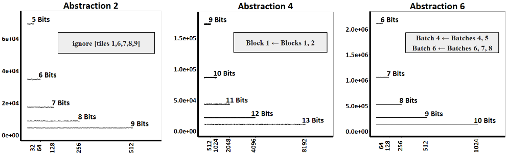
Before discussing the results of Table 1, we need to show the validity of our assumption that the distribution is uniform for the values in the lookup table of the ARHC implementation of our tested abstractions. Figure 2 shows these distributions for 3 of the 6 tested abstractions (the other 3 show similar behaviors). Each plot shows these distributions for 5 PPDBs of equal depth using 5 different numbers of bits per entry, i.e., 5 different values for c. The almost flat lines for each PPDB confirms our assumption that their distributions are uniform. We show the distribution of values in the lookup table rather than that of the heuristic values themselves. Recall that each heuristic value is calculated from three of the uniformly distributed table values. For values up to v, the calculated heuristic value is deterministic but for values greater than v, it is calculated as the sum of three values from a table where many values were chosen as random numbers uniformly distributed over the range 0 to 2b - 1.
A careful examination of columns 5 to 10 of Table 1 reveals that for all tested abstractions and PPDB sizes, ARHC PPDBs performed substantially better than similar sized Bloom PPDBs. The performance difference between the two approaches is quite substantial in almost every case. The Bloom approach expands between 1.4 and 11.3 times as many nodes as the ARHC approach. The Bloom approach also requires between 1.6 and 14.5 times as much time for problem solving. In 17 out of 18 cases, the Bloom approach requires more than twice as much time as the ARHC approach. The cases with the minimum and maximum ratios are bold-faced in Table 1. As well, the ARHC approach consistently provides a higher average heuristic value than the Bloom approach.
Construction time is another important efficiency criterion for every PDB representation or compression technique. The second column of Table 1 shows the construction time for each of the six abstractions with the ARHC and Bloom approaches. The construction time for the ARHC approach is between 1.4 and 2.3 times longer than for the Bloom approach. However, since the compressed PDB can be used for solving many problem instances, the ARHC construction time overhead can be amortized over many problem instances. For example, for Abstraction 1, the ARHC with the Small PPDB size has a construction time of 27 s that is negligible in comparison to the problem solving time of 2,028 s for 1,000 problem instances.
4.1 Discussion
In all experiments, the ARHC PPDB performed better than a similar sized Bloom PPDB. To get some intuition on why this is the case, consider a Bloom PPDB that keeps only the first depth with the desired false positive rate of 0.001. For a Bloom filter with 3 hash functions, 28 bits per entry are required to achieve this false positive rate. Even if we use say 8 hash functions, 14 bits per entry are still required to achieve a 0.001 false positive rate for a Bloom filter. However, with ARHC, which requires 3 hash functions, we only need 10 bits per entry to achieve a 0.001 false positive rate.
In a PPDBv implemented using the Bloom approach, information is lost by falsely assigning any heuristic value to a smaller value. However, in ARHC, we never lose any heuristic value information for values less than or equal to v. In other words, the only source of error in ARHC is assigning a lower heuristic value to an abstract state with an original heuristic value greater than v. Further, the amount of information lost for values greater than v in ARHC is just a function of the number of bits dedicated to each entry in the lookup table (this is due to uniform distribution of values in the ARHC lookup table achieved by initializing T randomly and also assigning random values to free vertices in the ARHC procedure). The free vertices are those vertices that can be assigned any value-in the range dedicated to each lookup entry-in the assigning step. In other words, if we hash an abstract state to three entries in the lookup table and all three are unassigned, two of them are free vertices and can be assigned any value in the appropriate range (if two are unassigned, one of them will be a free vertex). The random assignment of free vertices guarantees that we get a uniform distribution of their values in the assigning step. The error in a Bloom PPDB, however, cascades from level to level and requires more bits to recover from.
Finally, the PPDB approach for PDB compression has one important advantage over the min compression in general that makes it more applicable in practice. With min compression, we need to compute the original PDB and then compress it. In contrast, with PPDBs, we only need to compute the original PDB up to a certain depth. This is useful in cases where the original PDB does not fit in memory but the PPDB does. As an example, for the 2 abstractions of the Blocks World domain in the experimental results, the original PDB is so huge that we cannot compute it in the first place and therefore the min compression could not be used for those two cases.
5 Conclusions and FutureWork
We introduced ARHC, an efficient approach for lossy compression of PDBs with high compression rate and low heuristic information loss and the potential to lead to further improvements in combination with other compression strategies such as 1.6-bit pattern databases. It is domain-independent, effective, and addresses the weaknesses of the Bloom approach while maintaining its strengths. We showed that with the same compression rate, ARHC consistently performed better than the Bloom approach with respect to the average heuristic value, the number of nodes expanded using IDA* and the actual solution time. Our best results were achieved using the ARHC-Extended method.
To reduce information loss in a PPDBv, one could also merge some consecutive depths in the range [0,v] so that one could increase the number of values that represent v + 1. Preliminary experiments with this approach show notable improvements in both ARHC and Bloom PPDBs. The effectiveness of this merging strategy, however, is determined by a merge function that specifies which depths are merged together. Finding the best merge function in a domainindependent setting is not trivial and is the topic of future research.
@inproceedings{ijcai2017p611,
  title     = {Lossy Compression of Pattern Databases Using Acyclic Random Hypergraphs},
  author    = {Sadeqi, Mehdi and Hamilton, Howard J.},
  booktitle = {Proceedings of the Twenty-Sixth International Joint Conference on
               Artificial Intelligence, {IJCAI-17}},
  publisher = {International Joint Conferences on Artificial Intelligence Organization},
  editor    = {Carles Sierra},
  pages     = {4376--4383},
  year      = {2017},
  month     = {8},
  note      = {Main track},
  doi       = {10.24963/ijcai.2017/611},
  url       = {https://doi.org/10.24963/ijcai.2017/611},
}
TY - CPAPER TI - Lossy Compression of Pattern Databases Using Acyclic Random Hypergraphs AU - Sadeqi, Mehdi AU - Hamilton, Howard J. T2 - Proceedings of the Twenty-Sixth International Joint Conference on Artificial Intelligence, IJCAI-17 PB - International Joint Conferences on Artificial Intelligence Organization PY - 2017 SP - 4376 EP - 4383 DO - 10.24963/ijcai.2017/611 UR - https://doi.org/10.24963/ijcai.2017/611 ER -Copied
Machine-readable versions of this paper, for tools and AI agents:





