
Intelligent Belief State Sampling for Conformant Planning
Proceedings of the Twenty-Sixth International Joint Conference on Artificial Intelligence. Main track. Pages 4317-4323.
https://doi.org/10.24963/ijcai.2017/603
Keywords
- Planning and Scheduling: Conformant/Contingent planning
- Constraints and Satisfiability: Satisfiability
Abstract
We propose a new method for conformant planning based on two ideas. First given a small sample of the initial belief state we reduce conformant planning for this sample to a classical planning problem, giving us a candidate solution. Second we exploit regression as a way to compactly represent necessary conditions for such a solution to be valid for the non-deterministic setting. If necessary, we use the resulting formula to extract a counter-example to populate our next sampling. Our experiments show that this approach is competitive on a class of problems that are hard for traditional planners, and also returns generally shorter plans. We are also able to demonstrate unsatisfiability of some problems.
- [Albore et al., 2010] A. Albore, H. Palacios, and H. Geffner. Compiling uncertainty away in non-deterministic confor- mant planning. In Nineteenth European Conference on Artificial Intelligence (ECAI-10), 2010.
- [Albore et al., 2011] A. Albore, M. Ramírez, and H. Geffner. Effective heuristics and belief tracking for planning with incomplete information. In 21st International Confer- ence on Automated Planning and Scheduling (ICAPS-11), 2011.
- [Bonet and Geffner, 2000] B. Bonet and H. Geffner. Plan- ning with incomplete information as heuristic search in belief space. In Fifth International Conference on AI Plan- ning and Scheduling (AIPS-00), pages 52-61, 2000.
- [Brafman and Shani, 2012] R. Brafman and G. Shani. Re- planning in domains with partial information and sensing actions. Journal of Artificial Intelligence Research (JAIR), 45:565-600, 2012. IJCAI
- [Brafman and Shani, 2016] R. Brafman and G. Shani. On- line belief tracking using regression for contingent plan- ning. Artificial Intelligence (AIJ), 241:131152, 2016.
- [Bryce et al., 2006] D. Bryce, S. Kambhampati, and D. Smith. Planning graph heuristics for belief space search. Journal of Artificial Intelligence Research (JAIR), 26:35-99, 2006.
- [Castellini et al., 2003] C. Castellini, E. Giunchiglia, and A. Tacchella. SAT-based planning in complex domains: concurrency, constraints and nondeterminism. Artificial Intelligence (AIJ), 147:85-117, 2003.
- [Cimatti and Roveri, 2000] A. Cimatti and M. Roveri. Con- formant planning via symbolic model checking. Journal of Artificial Intelligence Research (JAIR), 13:305-338, 2000.
- [Clarke et al., 2000] E. Clarke, O. Grumberg, S. Jha, Y. Lu, and H. Veith. Counterexample-guided abstraction refine- ment. In Twelfth International Conference on Computer- Aided Verification (CAV-00), pages 154-169, 2000.
- [de Moura and Bjørner, 2008] L. de Moura and N. Bjørner. Z3: an efficient SMT solver. In Fourteenth International Conference on Tools and Algorithms for the Construc- tion and Analysis of Systems (TACAS-08), pages 337-340, 2008.
- [Ghallab et al., 2004] M. Ghallab, D. Nau, and P. Traverso. Automated planning: theory & practice. Elsevier, 2004.
- [Grastien and Scala, 2017] A. Grastien and E. Scala. Verify- ing the validity of a conformant plan is co-NP-complete, 2017. http://vixra.org/abs/1705.0340. Link
- [Grastien, 2015] A. Grastien. Self-healing as a combination of consistency checks and conformant planning problems. In 26th International Workshop on Principles of Diagnosis (DX-15), pages 105-112, 2015.
- [Haslum, 2012] P. Haslum. Incremental lower bounds for ad- ditive cost planning problems. In 22nd International Con- ference on Automated Planning and Scheduling (ICAPS- 12), 2012.
- [Helmert, 2006] M. Helmert. The fast downward planning system. Journal of Artificial Intelligence Research (JAIR), 26:191-246, 2006.
- [Hoffmann and Brafman, 2006] J. Hoffmann and R. Braf- man. Conformant planning via heuristic forward search: a new approach. Artificial Intelligence (AIJ), 170:507-541, 2006.
- [Hoffmann and Nebel, 2001] J. Hoffmann and B. Nebel. The FF planning system: Fast plan generation through heuris- tic search. Journal of Artificial Intelligence Research (JAIR), 14:253-302, 2001.
- [Kurien et al., 2002] J. Kurien, P. Nayak, and D. Smith. Fragment-based conformant planning. In Sixth Interna- tional Conference on AI Planning and Scheduling (AIPS- 02), pages 153-162, 2002.
- [Nguyen et al., 2012] K. Nguyen, V. Tran, T. Son, and E. Pontelli. On computing conformant plans using clas- sical planners: a generate-and-complete approach. In 22nd International Conference on Automated Planning and Scheduling (ICAPS-12), pages 190-198, 2012.
- [Palacios and Geffner, 2006] H. Palacios and H. Geffner. Compiling uncertainty away: solving conformant plan- ning problemsusing a classical planner (sometimes). In 21st Conference on Artificial Intelligence (AAAI-06), pages 900-905, 2006.
- [Palacios and Geffner, 2009] H. Palacios and H. Geffner. Compiling uncertainty away in conformant planning prob- lems with bounded width. Journal of Artificial Intelligence Research (JAIR), 35:623-675, 2009.
- [Rintanen, 2008] J. Rintanen. Regression for classical and nondeterministic planning. In Eighteenth European Con- ference on Artificial Intelligence (ECAI-08), pages 568- 572, 2008.
- [Seipp and Helmert, 2013] J. Seipp and M. Helmert. Counterexample-guided cartesian abstraction refinement. In 23rd International Conference on Automated Planning and Scheduling (ICAPS-13), 2013.
- [To et al., 2011] S. T. To, E. Pontelli, and T. C. Son. On the effectiveness of CNF and DNF representations in contin- gent planning. In 22nd International Joint Conference on Artificial Intelligence (IJCAI-11), pages 2033-2038, 2011. IJCAI
References were extracted automatically from the PDF and may contain errors.
Full text extracted automatically from the PDF; figures, tables and equations may differ. The PDF is the version of record.
1 Introduction
Conformant planning is the problem of finding a plan in an environment that is only partially known. In this work we restrict ourselves to uncertainty on the initial state and not in the actions' effects (or assume that this uncertainty can be integrated into the initial state).
We present a new approach to conformant planning. The approach is very similar to the CEGAR (counter-exampleguided abstraction refinement) technique used for modelchecking [Clarke et al., 2000] and in self-healing [Grastien, 2015]. The basic idea of CEGAR is to repeatly compute a solution to a simplified (abstracted) version of the problem at hand. If this solution is not correct for the original problem, it is analysed to enrich (refine) the simplified problem, so that a better solution can be generated at the next step of the procedure.
Practically we first assume we are given a set of "interpretations" of the initial belief state, i.e., some of the possible initial states. Each interpretation can be understood as a representative of one or several aspects, i.e., tag [Palacios and Geffner, 2006], of the conformant problem that the solver has to consider, e.g., the fact that an item that needs to be picked up could be in a given location. We reduce the problem of finding a conformant plan for this set of interpretations to classical planning, and solve it using an off-the-shelf planner.
We then use regression to efficiently determine whether this plan is incorrect for any initial state. If so, we extract one such state. This state is effectively a counter-example proving that the proposed plan is a non-conformant one. This state is then added to the current set of considered interpretations; this is how the set of interpretations (originally empty) is populated. This procedure guarantees that the interpretations are all relevant since they each contradict at least one of the plans generated earlier. For this reason we talk about "intelligent" sampling.
The paper presents CPCES, a conformant planner that is sound and complete, assuming sound and complete classical planner and regression procedures. If the underlying classical planner is optimal, then the resulting conformant planner also is. As far as we know, no previous work in the literature has looked at the conformant planning problem from this perspective. A side contribution is a verifier that decides whether a given plan is a solution to the conformant planning problem.
We test the planner on a large set of benchmarks. We notice that our planner is able to handle problems that are traditionally hard for existing planners, in particular problems with large "width". These results are very encouraging particularly given the simplicity of the approach, and the simplicity of the resulting developed software architecture. We took practically off-the-shelf a classical planner, i.e., FF [Hoffmann and Nebel, 2001] and a SAT-Solver, i.e., Z3 [de Moura and Bjørner, 2008] without any further tuning. We believe that the framework has a huge potential for a large class of conformant planning problems that are hard for current conformant planners. For instance, we are able to prove that some problem instances are unsatisfiable, i.e., there exists no conformant plan for these instances.
The present paper is organised as follows. After an intuitive presentation of our algorithm, we present the conformant planning problem. Then we present our approach, our conformant planning algorithm, and the theoretical properties it enjoys. The next two sections give more details on the two key components of our algorithm, namely the reduction from conformant planning to classical planning (given a small sample of the belief state) and the verification of a candidate plan which can lead to the generation of a counter-example. We discuss related works and finally we present experimental results.
2 Intuitive Explanation of CPCES
We start the paper with an intuitive explanation of our algorithm and why we expect our algorithm to perform well.
Consider the conformant planning domain known as ONEDISPOSE. This problem involves n objects in ℓ ≥ n locations. Each object ought to be moved to a specific location. Additional considerations include the facts that the agent must move between the locations; the initial location of these objects is unknown; the agent can only hold one object at a time; finally, since the problem is conformant, no observation is available. The optimal plan consists, for every object, in visiting all locations, trying to pick this object up, and dropping it at the right place (before moving to the next object).
Theoretically it is possible to enumerate all nℓ initial states and to compute a plan based on this set. Not all these states however are necessary to find an optimal plan. For each location consider the initial state in which all objects are in this location. From this subset of ℓ initial states one can infer that a conformant plan must try to pick every object up from every location, which is all the information we need to infer the optimal plan. Essentially this shows that we do not need all nℓ initial states but only ℓ states.
There remains the issue of how we determine the relevant initial states. The intuition is that we can compute a deterministic plan only from an incomplete set; then we can analyse such a plan to get the relevant states explaining why this plan is incorrect.
3 ProblemDefinition
Given a set of variables V we denote L(V ) the set of propositional formulas that only mention variables in V . A conformant planning problem is a tuple P = 〈F,A,ΦI,ΦG〉 where F is a finite set of state variables (or facts), A is a set of actions, ΦI ∈ L(F) is the initial formula, and ΦG ∈ L(F) is the goal formula. An action a ∈ A is a pair 〈p, eff 〉 where p ∈ L(F) is a precondition and eff is the effects of the action. The effects are a function that associates each literal ℓ ∈ F ∪ {¬f | f ∈ F} to a condition eff (ℓ) ∈ L(F). To simplify later notations, we assume that the conditions of a literal and its negation are mutually inconsistent: eff (f) ∧ eff (¬f) |= ⊥. 1
Informally, the initial state is one of the Boolean assignments of the facts that satisfy the initial formula. An action is applicable in a state if its precondition is satisfied in the state. Each fact f is true after the action if eff (f) holds in the current state or f was already true and eff (¬f) does not hold (cf. Eq. (2) below). A goal state is a state that satisfies the goal formula.
Our formal definition of the semantics of the conformant problem avoids the direct use of states, but it is equivalent to the standard one. A belief state B ∈ L(F) is a propositional formula (ΦI is such a belief state). Action a = 〈p, eff 〉 is applicable in belief state B if B |= p. The result of applying
1 This assumption is not restrictive as conflicting conditions can be avoided by integrating them to the precondition of the action.
where Ta is the transition function defined by
In this formula, F ′ is a copy of the variables in F that is used to reason about the belief states before and after the action. ∃V. is the existential operator (i.e., the value of the variables of V , here the facts before the action, is forgotten). [F/F ′ ] is the operator that switches the value of the variables F and F ′ so that: f[F/F ′ ] represents a set of transitions where the target set is defined by f being true (the origin set is free); (∃F.set-of-transitions)[F/F ′ ] represents the target states of the specified set of transitions.
A plan π = a1, . . . , ak is a (possibly empty) sequence of actions. The application B[π] of the plan is the incremental application: B[a1] . . . [ak]. The plan is applicable if each of its actions ai is applicable in B[a1] . . . [ai-1].
A solution to the planning problem is a plan π that is applicable fromΦI and that leads to the goal set: ΦI[π] |= ΦG; we write Π(P) the set of solutions to the planning problem P. A solution is optimal if there is no shorter solution.
A state of a belief is a model satisfying the belief. The set of states of belief state B is denoted by states(B). A planning problem is deterministic if it has a single initial state. Deterministic (aka classical) problems are generally easier to solve than non-deterministic (aka conformant) ones.
4 Our Approach
We now present the theoretical foundation of our approach and the conformant planning algorithm that we derive from it. The specifics of the two main methods used in this algorithm, namely the reduction of a simplified conformant planning problem to classical planning and the computation of a counter-example, are detailled in the next sections.
We will compute a conformant plan using only a subset of the initial states (which will allow us to reduce the problem to classical planning). Practically this means that we are given a belief state that entails the initial belief state of the problem: B |= ΦI. We write PB the planning problem defined by P except that the initial formula is replaced by B.
The central property that underpines all the results in this section is the following trivial property:
Proposition 1 The following proposition holds
A consequence of Proposition 1 is that B |= ΦI implies that Π(P) is a subset of Π(PB). In other words it is possible to reason about the problem PB without missing any plan. A solution for problem PB may however not be a solution to P.
Assume now that a solution π for PB has been computed. We are interested in deciding whether π is indeed a solution for P. A counter-example of initial formula ΦI for plan π is a state q ∈ states(ΦI) such that π does not belong to the set Π(Pq). The following result is essential to prove the properties of the algorithm and can be derived from Proposition 1.
Proposition 2 Let π be a solution for PB that is not a solution for P. Then there exists at least one counter-example of ΦI for π. Furthermore none of these counter-examples q belongs to B (q ̸∈ states(B)) and π is not a solution for PB∨q.
We can therefore verify whether a solution for B is a solution for ΦI by searching for counter-examples. It is then sensible to add the counter-example to the belief state since this means that the plan that will be computed for the new belief state will not include the plan that was just disproved.
These propositions lead us to Algorithm 1. We start with an empty belief state B := ⊥. At each iteration we compute a plan π for the current belief state; if π is correct for P then we return this plan; otherwise we extract a counter-example and add it to the belief state.
Algorithm 1 Conformant Planning Algorithm.
1: input: planning problem P 2: B := ⊥ {Initial sample of the belief state} 3: π := ε {Empty plan-is a plan for belief state ⊥} 4: loop 5: if π is a solution for P then 6: return π {Plan found} 7: end if 8: Let q be a counter-example 9: B := B ∨ q 10: Compute new plan π for PB 11: if no such π exists then 12: return no plan exists 13: end if 14: end loopWe can now prove properties of this algorithm.
Lemma 1 Algorithm 1 is sound and complete (if the subroutines that compute a counter-example and a classical plan are sound and complete).
First, the plan returned by the algorithm has been verified for P and is therefore correct. Second, assume that the algorithm returns that there is no plan; then there is no plan for B; however since B is a collection of counter-examples, then B |= ΦI and Π(P) ⊆ Π(PB) = ∅; hence there is no plan. Finally, each iteration adds a new state to B and, since the number of initial state is finite, the algorithmwill terminate.
Lemma 2 If the planner used in Algorithm 1 is optimal, then Algorithm 1 is optimal.
Proof: Because Π(PB) is a superset of Π(P) it contains the optimal plan for Π(P), too. Therefore if the optimal plan of the former belongs to the later, it is an optimal solution for the conformant problem.
The next sections concentrate on the two subroutines of Algorithm 1: the computation of a plan for B through a reduction to classical planning and the computation of a counterexample through regression.
5 Reduction fromConformant Planning to Classical Planning
In this section we assume given a belief state B. It is assumed here that states(B) is fairly small (no more than a few hundreds elements) as this method becomes impractical for larger belief states. The experiments demonstrate that we are often able to find a plan before this assumption gets violated.
Our reduction of conformant planning is similar to that of Palacios and Geffner (2009). However they used a merge action that we do not require.
Let {q1, . . . , qk} = states(B) be the set of states of B. Remember that each qi is a formula. The reduction consists in running k planning problems in parallel where all actions are synchronised. To echo the notation from Palacios and Geffner we define facts f/qi that indicate that the fact f is true under the initial state interpretation qi. We write F/qi the set of facts derived for interpretation qi from the set F.
Definition 1 Given a set of states states(B) = {q1, . . . , qk} the reduction of conformant planning problem PB = 〈F,A, B,ΦG〉 is the deterministic planning problem red(PB) = 〈F ′ , A′ , B′ , Φ′G 〉 where
- F ′ = F/q1 ∪ · · · ∪ F/qk ,
- A′ = {red(a) | a ∈ A} where red(〈p, eff 〉) = 〈p′ , eff ′ 〉 is defined by p′ = ∧i∈{1,...,k} p[F/F/qi ] and eff ′ is such that eff ′ (ℓ/qi ) = eff (ℓ)[F/F/qi ],
- B′ = ∧i∈{1,...,k} qi[F/F/qi ], and
- Φ′G = ∧i∈{1,...,k} ΦG[F/F/qi ].
The reduction of action a can be explained as follows: red(a) is applicable if p is satisfied under all interpretations; the effect ℓ applies for an interpretation qi if its condition eff (ℓ) is satisfied for this interpretation. The initial belief state is the description of the facts that hold under each interpretation. All interpretations must satisfy the goal condition in the goal state.
Lemma 3 A plan π = a1, . . . , an is a solution to PB iff the plan red(a1), . . . , red(an) is a solution to red(PB).
Lemma 3 proves that the reduction from conformant planning to classical planning is correct. A classical planner can therefore be used to compute a plan for PB.
Notice that this reduction does not increase the number of actions; therefore the branching factor of the planning problem PB does not increase with the size of B. It increases however the number of facts linearly in the number of states in B, and similarly increases the number of conditional effects of each action.
6 Computing a Counter-Example
We now want to verify if a given plan is a solution to the planning problem, and generate a counter-example when it is not. Verification of conformant plan π = a1, . . . , ak can be performed by computing the regression of the plan, i.e., the weakest precondition on the initial set that guarantees that π is a solution. Formally the regression of π from ΦG is the (unique) maximal belief state Reg(π,ΦG) such that π is a solution to PReg(π,ΦG). How to compute the regression is well-known [Rintanen, 2008; Brafman and Shani, 2016]. The set of counter-examples is then given by ΦI ∧ ¬Reg(π, ΦG).
Instead of computing Reg(π,ΦG) explicitly however we generate a SAT problem, all models of which is a counterexample. The reduction to SAT is fairly straightforward.
The SAT problem searches for a sequence of states q0, . . . , qk. Firstly a set of constraints based on Tai ensures that q1, . . . , qk are the states reached by applying the actions a1, . . . , ak in this order assuming all actions are applicable. Remember that at his stage, as opposed to SAT-based classical planning, the plan π = a1, . . . , ak is known. Secondly for all index i, a Boolean variable pi is added that evaluates to true iff the action ai is applicable in qi-1. Thirdly a set of constraints ensures that the plan is not a solution for q0, i.e., either the final state is not a goal state or one of the action is not applicable: (¬p1) ∨ . . . ∨ (¬pk) ∨ ¬ΦG[F/Fk]. Finally a set of constraints ensures that q0 is an initial state.
It is easy to show the following result:
Lemma 4 The set of satisfying assignments to the SAT problem described above is the set of counter-examples of π.
The decision problem associated with the detection of counter-examples is CO-NP-COMPLETE [Grastien and Scala, 2017], which justifies the use of SAT techniques. Our reduction to SAT mimics the one used in SAT-based classical planning except that the initial state, rather than the plan, is unknown. The number of free variables in our SAT problem is therefore smaller and the problem is quite simple to solve.
7 RelatedWorks
Conformant planning was quickly characterised and solved as a search problem over the space of belief states [Bonet and Geffner, 2000]. The representation of these belief states has however been identified as one bottleneck. Different techniques have been used to address this issue such as using BDDs [Cimatti and Roveri, 2000] or representing the belief state implicitely by the prefix of the plan [Hoffmann and Brafman, 2006; To et al., 2011].
A different approach [Palacios and Geffner, 2009; Albore et al., 2010] consists in reducing the conformant planning problem to a classical planning one where every literal f is replaced by the literals Kf and K¬f that indicate that f is known to be true or false (the effects of the actions are changed accordingly). This translation is not sufficient to guarantee completeness however, and tags and merges have been introduced for this purpose. A tag is a proposition that is satisfied by some initial states and a merge is a collection of tags, one of each is satisfied by any initial state. The classical planning problem is augmented to include facts of the form KL/t, where L is a literal and t a tag, with the semantics "L is known to be true if t held in the initial state." When KL/t is true in a state for all t in a given merge, then KL is added to the state. It is possible to automatically compute the list of tags and merges that are required to guarantee soundness and completeness of this approach.
Tags can be seen as the kernel of a counter-example, the core reason (or one of the core reasons) why some plans are not solutions. Computing all merges upfront guarantees that all "contingencies" will be considered by the classical planner. Completeness however is only guaranteed when all relevant tags and merges are computed. Their number is exponential in the width of the conformant planning problem, which limits this approach to domains where the width is small (as shown in the experiments).
Palacios and Geffner (2009) also introduced the notion of basis, a subset of initial states that is guaranteed to have the same set of plans as the initial belief states: Π(P) = Π(PB). A sound and complete conformant planning method consists in first computing a basis B, and second computing a solution to PB by reduction to classical planning. This method is practical if the basis is small.
The basis is guaranteed to represent the exact same set of plans as the initial belief state; in comparison we only require a sampling such that the planner returns a valid plan for the initial belief state. Our requirement is weaker than the requirement for a basis, which means that we will generally produce a much smaller belief state. In the optimal setting for instance, it is unnecessary to find counter-examples for suboptimal plans.
Notice also that we compute our sampling incrementally while the basis is computed upfront. This means that the basis must be computed in a very conservative way, i.e., by including states that could not be proved to be unnecessary.
Other methods have used sampling for conformant planning, but our objective is different from theirs. The purpose of these samplings is generally to produce heuristics in a belief space search [Bryce et al., 2006] while we only sample the initial state. There has been other test and generate approaches to conformant planning [Kurien et al., 2002; Castellini et al., 2003]. These approaches did not incrementally generate counter-examples to ensure that better plans are produced over time.
Another approach that uses sampling is Sample, Determinize, Replan [Brafman and Shani, 2012]. SDR computes a plan from a single initial state, executes and monitors it (it assumes partial observability), and replans when the execution failed. In comparison we search for risks of failure before execution, and we compute a completely new plan. Since we replan without knowing for sure that the current state is not the one we planned for, we also need to remember all the counter-examples we generated.
8 Implementation and Experimental Analysis
8.1 Implementation
In order to study the benefits, the drawbacks, and the computational implications of the approach presented in this paper, we used a classical planner and a SAT-Solver and implemented in Java a module that orchestrates the interactions between these two components. The classical planner used is FAST FORWARD (FF) [Hoffmann and Nebel, 2001]. FF is a pure classical planner based on heuristic search. The planner has been the winner of many competitions throughout the last decade and is one of the most robust and efficient planning system. The SAT-Solver is Z3, a state of the art theorem prover [de Moura and Bjørner, 2008].
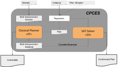
(:action drop :parameters (?o - obj ?p - pos ) :precondition (forall (?i - inter) (and (located ?p ?i) (trash_at ?p ?i))) :effect (and (forall (?i - inter) (when (holding ?o ?i) (and (not (holding ?o ?i)) (disposed ?o ?i))))))Figure 1 reports the developed architecture. Note here that our system does not make any assumptions on the solvers being used. The interactions between the various modules have been done using PDDL to represent the planning problems, and SMT-LIB 2 to represent the formula.
PDDL [Ghallab et al., 2004] is the de-facto language to represent planning problems in a succinct way. Actions are represented in a schematic form, and the planner is in charge of grounding them against the current instance. To make the introduction of new samples operative within the planning problem we allow the introduction of special types of object, namely inter. Each of these objects captures a specific interpretation of our initial state. Each predicate of our planning domain is then extended with the inter parameter. This way, the grounding of each predicate is not only a function of the actual objects present in the conformant problem, but also a function of the current interpretations we are considering in our reduction to classical planning. This effectively adds a new dimension to the problem, orthogonal to and somehow separated from the other aspects of the conformant problem.
Following the reduction presented earlier, we use the ?inter object in our action schema, too. Every action is lifted by one level by quantifying every precondition formula and every effect over all the possible interpretations. This ensures that the action is applied iff each of the possible interpretation satisfies its precondition. And analogously for the effects. Figure 2 reports an example for the Drop action in the DISPOSE domain. This schema of translation has two main benefits: i) it allows to construct the domain theory just once in our algorithm; the actual grounding of the actions will depend on the number of objects instantiated in the problem file;
2 http://smtlib.cs.uiowa.edu/
ii) it preserves to some extent the structural information peculiar to the conformant setting. As a matter of fact the problem grows incrementally only in one dimension, which is the one mirroring the uncertainty to be handled in that particular problem. We believe it is important to keep track of this structural information that can be exploited by the classical planner.
Our system is called CPCES (Conformant Planner via Counter Example and Sampling) 3 . Its architecture has been conceived to be modular and independent from the particular solvers. This means that the methodology hereby presented can benefit from any advance in the classical planning and satisfiability contexts. For instance we have tried other planners that are able to handle conditional effects and quantification, (e.g., FAST-DOWNWARD [Helmert, 2006]). FF is the only classical planning system able to efficiently deal with quantification and conditional effects altogether. The FASTDOWNWARD translator suffers of some severe computational issue, probably due the grounding and translation to SAS+ which is implemented in Python. Unfortunately, most stateof-the-art planners use such a translator as pre-processor. We chose the SAT-Solver Z3 because the input language (SMTLIB) is easier to interpret and manipulate above all when CPCES has to iterate over the counter-examples, or the user wants to understand the reasons why the current plan is incorrect. The experiments show that the time used by the SATSolver is a small percentage of the total time.
8.2 Domains
We took a set of domains fromAlbore et al. [2011]. In particular we focus our attention on two categories: domains having width strictly larger than 1 that are notoriously difficult for all the state of the art planning systems, and domains with a width less than or equal 1.
The first set of domains consists of BLOCKSWORLD, RAO'S KEYS, ONE-DISPOSE and LOOK-GRAB. As we will see, none of the planners we are aware of has been able to efficiently solve those instances, or to prove their unsolvability.
In the second set of domains we consider: DISPOSE, BOMB, COINS and UTS. Planners developed in the literature are able to handle those domains quite well.
In the next two subsections we look at how CPCES compares against T1, a very fast heuristic search planner. Our analysis is meant to study the capability of systems to produce sound plans of reasonable length. In this paper we left out from the comparison GC-LAMA [Nguyen et al., 2012] for two main reasons: i) we are not sure of the soundness of the produced plans, and ii) the length of the plans produced by GC-LAMA is often magnitude longer than the ones we obtain. GC-LAMA has been reported to produce a plan for the fourth instance of BLOCKSWORLD which is unsolvable, as well as the fourth instance of RAO'S KEYS. We leave this analysis as a future work, and we focus on comparing our planner with T1 instead.
| Coverage | Length | Time | ||||
|---|---|---|---|---|---|---|
| Domain | CC | T1 | CC | T1 | CC | T1 |
| BOMB(9) | 8 | 9 | 136.0 | 130.5 | 102.7 | < 1 |
| COINS(9) | 8 | 9 | 81.3 | 140.2 | 8.8 | < 1 |
| DISPOSE(11) | 5 | 8 | 210.4 | 246.2 | 321.2 | 10.1 |
| UTS(15) | 14 | 14 | 53.9 | 63.6 | 65.6 | 4.6 |
| BLOCKSWORLD(4) | 4 | 2 | 12.5 | 13.0 | < 1 | < 1 |
| RAO'S KEYS(3) | 3 | 1 | 16.0 | 21.0 | < 1 | < 1 |
| ONE-DISPOSE(10) | 6 | 4 | 67.5 | 79.3 | 13.3 | 202.2 |
| LOOK-GRAB(18) | 18 | 15 | 50.9 | 33.7 | 28.5 | 129.8 |
| Total | 66 | 62 | ||||
8.3 Experimental Results
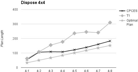
Table 1 reports the data collected for the two systems across many instances of the aforementioned domains, where we compared coverage, plan-quality and run-time spent to find a solution. Experiments confirmed our intuition. CPCES does not directly suffer from the particular structure of the problem. For this reason its performances are independent from the particular width of the problem. It is not the case for T1 though. This results in an overall higher coverage for CPCES (66 over 62) but more importantly the two systems seem to behave well on two different dimensions. CPCES is in fact substantially slower than T1 on the 1-width domains, although it produces plans whose quality is (apart from BOMB) consistently better than T1. On the other hand, CPCES outperforms T1 on the more complex domains whilst keeping the average plan length competitive with T1 (making exception for LOOK-GRAB). T1 shows performances that are typical of a very greedy heuristic search planner, i.e., it either finds a plan in a few seconds, or it does not find a plan at all. CPCES instead adopts a more systematic approach, thus performing quite consistently across a large variety of problems. Finally, in our setting we are not using an optimal planner (even though we could), though the plans in some domain turned out to be of very good quality. This is an effect of the underlying incremental lower bounding given by our architecture. As a demonstration of this, have a look at Figure 3, where CPCES, T1, and the ideal optimal planner are compared across instances from the DISPOSE domain.
Table 2 reports data investigating some of the behavior of our system on the most difficult (solved) instances across the tested domains. Unsurprisingly, apart for the smaller instances, the majority of the computational time spent for each instance is due to the classical planner. The planner computes, for each new sample generated, a plan of increasing size. For some bigger instances this becomes the bottleneck of our approach. The other component being evaluated is the SAT-Solver, in our case Z3. As it is possible to note from the table, the computational time devoted to this task barely reaches 7% in BOMB-100-5. The remaining computational part is spent doing regression and the machinery built to accommodate the interactions between these modules.
3 The system is available at https://bitbucket.org/ enricode/cpces
| Planner | SAT | Samples | T | |
|---|---|---|---|---|
| BLOCKSWORLD-03 | 0.2 | 0.9 | 25 | 4.4 |
| RAO'S KEYS-03 | 0.1 | 0.2 | 21 | 1.9 |
| BOMB-100-5 | 116.9 | 10.8 | 106 | 159.3 |
| COINS-20 | 5.2 | 1.9 | 43 | 14.1 |
| DISPOSE-8-2 | 1347.5 | 48.2 | 129 | 1508.4 |
| UTS-k-50 | 758.3 | 11.3 | 74 | 800.6 |
| ONE-DISPOSE-5-2 | 402.6 | 8.6 | 92 | 437 |
| LOOK-GRAB-8-3-3 | 11.8 | 1.5 | 11 | 19.6 |
Another interesting and key factor in these experiments is the number of samples to generate. This number represents the actual space of interpretations that we needed to explore to handle the uncertainty in the initial state. For instance, in DISPOSE we have 64 × 64 possible initial states. The incremental sampling here allows us to use just 64 + 64 + 1 counter-examples generated from the starting empty plan.
9 Conclusion
We presented a new approach to conformant planning that is conceptually very simple and that shows a lot of promise. With this method we were able to solve a class of problems that have traditionally been considered hard (problems with a width greater than one). Furthermore the solutions found by our planner are generally shorter than other solvers.
In the context of deterministic planning the CEGAR approach, i.e., the approach where counter-examples are used to identify important pieces of information in the problem description, has been investigated [Seipp and Helmert, 2013; Haslum, 2012]. In this paper we show that it may substantially benefit the understanding and the development of more expressive planning problems as well.
@inproceedings{ijcai2017p603,
  title     = {Intelligent Belief State Sampling for Conformant Planning},
  author    = {Grastien, Alban and Scala, Enrico},
  booktitle = {Proceedings of the Twenty-Sixth International Joint Conference on
               Artificial Intelligence, {IJCAI-17}},
  publisher = {International Joint Conferences on Artificial Intelligence Organization},
  editor    = {Carles Sierra},
  pages     = {4317--4323},
  year      = {2017},
  month     = {8},
  note      = {Main track},
  doi       = {10.24963/ijcai.2017/603},
  url       = {https://doi.org/10.24963/ijcai.2017/603},
}
TY - CPAPER TI - Intelligent Belief State Sampling for Conformant Planning AU - Grastien, Alban AU - Scala, Enrico T2 - Proceedings of the Twenty-Sixth International Joint Conference on Artificial Intelligence, IJCAI-17 PB - International Joint Conferences on Artificial Intelligence Organization PY - 2017 SP - 4317 EP - 4323 DO - 10.24963/ijcai.2017/603 UR - https://doi.org/10.24963/ijcai.2017/603 ER -Copied
Machine-readable versions of this paper, for tools and AI agents:





