
Locality Preserving Projections for Grassmann manifold
Proceedings of the Twenty-Sixth International Joint Conference on Artificial Intelligence. Main track. Pages 2893-2900.
https://doi.org/10.24963/ijcai.2017/403
Keywords
- Machine Learning: Unsupervised Learning
- Machine Learning: Machine Learning
Abstract
Learning on Grassmann manifold has become popular in many computer vision tasks, with the strong capability to extract discriminative information for imagesets and videos. However, such learning algorithms particularly on high-dimensional Grassmann manifold always involve with significantly high computational cost, which seriously limits the applicability of learning on Grassmann manifold in more wide areas. In this research, we propose an unsupervised dimensionality reduction algorithm on Grassmann manifold based on the Locality Preserving Projections (LPP) criterion. LPP is a commonly used dimensionality reduction algorithm for vector-valued data, aiming to preserve local structure of data in the dimension-reduced space. The strategy is to construct a mapping from higher dimensional Grassmann manifold into the one in a relative low-dimensional with more discriminative capability. The proposed method can be optimized as a basic eigenvalue problem. The performance of our proposed method is assessed on several classification and clustering tasks and the experimental results show show its clear advantages over other Grassmann based algorithms.
- [Absil et al., 2008] P.-A. Absil, Robert Mahony, and Rodolphe Sepulchre. Optimization Algorithms on Matrix Manifolds. Princeton University Press, 2008.
- [Bishop, 2006] Christopher M. Bishop. Pattern Recognition and Machine Learning (Information Science and Statis- tics). Springer-Verlag New York, Inc., Secaucus, NJ, USA, 2006.
- [Chen et al., 2007] Sibao Chen, Haifeng Zhao, Min Kong, and Bin Luo. 2D-LPP: A two-dimensional extension of locality preserving projections. Neurocomputing, 70:912- 921, 2007.
- [Comon, 1994] Pierre Comon. Independent component anal- ysis, a new concept? Signal Processing, 36(3):287-314, 1994.
- [Faraki et al., 2015] Masoud Faraki, Mehrtash T. Harandi, and Fatih. Porikli. More about VLAD: A leap from Eu- clidean to Riemannian manifolds. In CVPR, 2015.
- [Hamm and Lee, 2008] Jihun Hamm and Daniel D. Lee. Grassmann discriminant analysis: a unifying view on sub- space-based learning. In ICML, 2008.
- [Harandi et al., 2011] Mehrtash T. Harandi, Conrad Sander- son, Sareh Shirazi, and Brian C. Lovell. Graph embedding discriminant analysis on Grassmannian manifolds for im- proved image set matching. In CVPR, 2011.
- [Harandi et al., 2013] Mehrtash T. Harandi, Conrad Sander- son, Chunhua Shen, and Brain C. Lovell. Dictionary learn- ing and sparse coding on Grassmann manifolds: An extrin- sic solution. In ICCV, 2013.
- [Harandi et al., 2014] Mehrtash T. Harandi, Mathieu Salz- mann, and Richard Hartley. From manifold to manifold: Geometry-aware dimensionality reduction for SPD matri- ces. In ECCV, 2014.
- [Harandi et al., 2015] Mehrtash T. Harandi, Richard Hartley, Brian Lovell, and Conrad Sanderson. Sparse coding on symmetric positive definite manifolds using Bregman di- vergences. IEEE TNNLS, 27(6):1294-1306, 2015.
- [He and Niyogi, 2003] Xiaofei He and Partha Niyogi. Lo- cality preserving projections. In NIPS, 2003.
- [He et al., 2005] Xiaofei He, Deng Cai, Shuicheng Yan, and Hongjiang Zhang. Neighborhood preserving embedding. In ICCV, 2005.
- [Huang et al., 2014] Zhiwu Huang, Ruiping Wang, Shiguang Shan, and Xilin Chen. Learning Euclidean- to-Riemannian metric for point-to-set classification. In CVPR, 2014.
- [Huang et al., 2015] Zhiwu Huang, Ruiping Wang, Shiguang Shan, and Xilin Chen. Projection metric learning on Grassmann manifold with application to video based face recognition. In CVPR, 2015.
- [Jayasumana et al., 2015] Sadeep Jayasumana, Richard Hartley, Mathieu Salzmann, Hongdong Li, and Mehrtash T. Harandi. Kernel methods on Riemannian manifolds with Gaussian RBF kernels. IEEE PAMI, 37(12):2464-2477, 2015.
- [Ju et al., 2015] Fujiao Ju, Yanfeng Sun, Junbin Gao, Yongli Hu, and Baocai Yin. Image outlier detection and feature extraction via L1-norm based 2D probabilis- tic PCA. IEEE TIP, 24(12):4834-4846, 2015.
- [Kvalseth, 1987] Tarald O. Kvalseth. Entropy and correla- tion : Some comments. IEEE TSMC Part C, 17(3):517- 519, 1987.
- [Luo et al., 2016] Minnan Luo, Feiping Nie, Xiaojun Chang, Yi Yang, Alexander Hauptmann, and Qinghua Zheng. Avoiding optimal mean robust PCA/2DPCA with non- greedy ℓ 1 -norm maximization. In IJCAI, 2016.
- [Nguyen et al., 2008] Nam Nguyen, Wanquan Liu, and Svetha Venkatesh. Ridge regression for two dimensional locality preserving projection. In ICPR, 2008.
- [Pennec et al., 2006] Xavier Pennec, Pierre Fillard, and Nicholas Ayache. A Riemannian framework for tensor computing. IJCV, 66(1):41-66, 2006.
- [Sun et al., 2010] Liang Sun, Betul Ceran, and Jieping Ye. A scalable two-stage approach for a class of dimensionality reduction techniques. In KDD, 2010.
- [Turaga et al., 2011] Pavan Turaga, Ashok Veeraraghavan, Anuj Srivastava, and Rama Chellappa. Statistical com- putations on Grassmann and Stiefel manifolds for image and video-based recognition. IEEE TPAMI, 33(11):2273- 2286, 2011.
- [Wang and Gao, 2016] Qianqian Wang and Quanxue Gao. Robust 2DPCA and its application. In CVPR, 2016.
- [Wang et al., 2008] Haixian Wang, Sibao Chen, Zilan Hu, and Bin Luo. Probabilistic two-dimensional principal component analysis and its mixture model for face recog- nition. Neural Computing and Applications, 17(5-6):541- 547, 2008.
- [Wang et al., 2012] Rruiping Wang, Huimin Guo, LArry S. Davis, and Qionghai Dai. Covariance dis- criminative learning: A natural and efficient approach to image set classification. In CVPR, 2012.
- [Wang et al., 2016] Boyue Wang, Yongli Hu, Junbin Gao, Yanfeng Sun, and Baocai Yin. Product Grassmann mani- fold representation and its LRR models. In AAAI, 2016.
- [Xie et al., 2016] Liping Xie, Dacheng Tao, and Haikun Wei. Multi-view exclusive unsupervised dimension reduction for video-based facial expression recognition. In IJCAI, 2016. IJCAI
- [Xu et al., 2009] Yong Xu, Ge Feng, and Yingnan Zhao. One improvement to two-dimensional locality preserving pro- jection method for use with face recognition. Neurocom- puting, 73(2009):245-249, 2009.
- [Yang et al., 2004] Jian Yang, David Zhang, Alejandro F. Frangi, and Jing-yu. Yang. Two dimensional PCA: A new approach to appearance-based face representation and recognition. IEEE TPAMI, 26(1):131-137, 2004.
References were extracted automatically from the PDF and may contain errors.
Full text extracted automatically from the PDF; figures, tables and equations may differ. The PDF is the version of record.
1 Introduction
Dimensionality reduction (DR), which extracts a small number of features from original data by removing redundant information and noise, can improve efficiency and accuracy in a wide range of applications, involving facial recognition [He et al., 2005; Xie et al., 2016], feature extraction [Luo et al., 2016; Wang and Gao, 2016] and so on. The classic DR algorithms include Locality Preserving Projections (LPP) [He et al., 2005], Principal Components Analysis (PCA) [Bishop, 2006], Canonical Correlation Analysis (CCA) [Sun et al., 2010] and Independent Component Analysis (ICA) [Comon, 1994]. Most existing DR algorithms are mainly designed to work with vector-valued data, which cannot be directly applied on multi-dimensional data or structured data (i.e., matrices, tensors). Simply vectorizing such structured data to fit vector-based DR algorithms may destroy valuable structural and/or spatial information hidden in data. Therefore, how to effectively and properly reduce the dimensionality of structured data becomes an urgent issue in the big data era.
∗Corresponding author: Yongli Hu (huyongli@bjut.edu.cn). Yongli Hu, Yanfeng Sun and Baocai Yin are also with Beijing Advanced Innovation Center for Future Internet Technology. Muhammad Ali is with Charles Sturt University, Bathurst, Australia.
In practical application tasks such as those in computer vision, except for well-structured data like matrices or tensors, there exist data which are manifold-valued. For example, in computer vision, the movement of scattered keypoints in images can be described by subspaces, i.e., the points on the so-called Grassmann manifold [Absil et al., 2008]; and the covariance feature descriptors of images are SPD manifold-valued data [Pennec et al., 2006]. How to design learning algorithms for these two types of special manifold-valued data has attracted great attention in the past two decades [Huang et al., 2014; Faraki et al., 2015; Jayasumana et al., 2015]. For our purpose in this paper, we will briefly review some recent progress about DR algorithms for structured and manifold-valued data.
For a clear outline, we start with PCA. PCA is the most commonly used DR algorithm for vectorial data. The basic idea of PCA is to find a linear DR mapping such that as much variance in dataset as possible is retained. The classic PCA has been extended to process two dimensional data (matrices) directly with great success [Yang et al., 2004] (2DPCA). Wang et al. [2008] consider the probabilistic 2DPCA algorithm including the algorithm for the mixture of local probabilistic 2DPCA. To identify outliers in structured data, Ju et al. [2015] introduce the Laplacian distribution into the probabilistic 2DPCA algorithm.
Contrary to the global variance constraint in PCA-alike algorithms, LPP focuses on preserving the local structure of original data in the dimension-reduced space. The first work of extending LPP for 2D data was proposed in [Chen et al., 2007], which is operated directly on image matrices. The experimental results show that 2DLPP performs better than 2DPCA and LPP. Xu et al. [2009] propose a supervised 2DLPP by constructing a discriminative graph of labeled data. To reduce the high computational cost of 2DLPP, Nyuyen et al. [2008] improve 2DLPP by using the ridge regression.
However, the aforementioned DR algorithms for matrices are concerned in terms of Euclidean alike distance. Although the Riemannian structure has been shown to overcome the limitations of Euclidean geometry of data [Pennec et al., 2006; Hamm and Lee, 2008], the computational cost of the resulting techniques increases substantially with the increasing dimensionality of manifolds (i.e., the dimension of its embedding space). To the best of our knowledge, few attention has been paid on DR for Riemannian manifold.
Harandi et al. [2014] extend PCA onto SPD manifold by employing its Riemannian metrics, and then incorporate a discriminative graph of the labeled manifold data to achieve a supervised DR algorithm for SPD manifold. Recent research has shown that the Grassmann manifold, another type of Riemannian matrix manifold, is a good tool to represent videos or imagesets [Wang et al., 2012; Harandi et al., 2013; Harandi et al., 2015; Wang et al., 2016]. In a newly proposed supervised metric learning on the Grassmann manifold [Huang et al., 2015], an orthogonal matrix that maps the original Grassmann manifold into a more discriminative one is learned from data. In handling Grassmann-valued data, one usually employs one of three ways: embedding into a Hilbert feature space defined a Grassmann kernel function [Harandi et al., 2011]; or embedding into the symmetric matrix manifold (a plain Euclidean space) [Wang et al., 2016]; or projecting data onto tangent spaces (extrinsic way) [Harandi et al., 2013]. However the performance of all these ways can be hindered by the high dimensionality of given Grassmann manifold. It has become critical to reduce the dimensionality of Grassmann data.
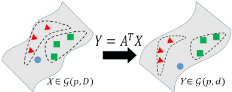
Motivated by [Huang et al., 2015], we learn a projected matrix to reduce the dimensionality of Grassmann manifold in this paper. To fulfill the goal, we extend LPP local criterion onto Grassmann manifold through embedding Grassmann manifold into a symmetric matrices space [Harandi et al., 2013] such that the local structure of original Grassmann data can be well preserved in the newly projected Grassmann manifold. Figure 1 illustrates that a projected matrix A is introduced to map the original high-dimensional Grassmann manifold into the one in a relative low-dimensional with more discriminative capability, which still preserves the structure of original Grassmann points.
The contribution of this paper is summarized as follows,
- A novel unsupervised DR algorithm in the context of Grassmann manifold is introduced. The DR is imple-
mented by learning a mapping to a Grassmann manifold in a relative low-dimensional with more discriminative capability;
- The proposed method generalizes the classic LPP framework to non-Euclidean Grassmann manifolds and only involves the basic eigenvalue problem; and
We briefly review some necessary knowledge about LPP and Grassmann manifold in next section.
2 Backgrounds
2.1 Locality Preserving Projections (LPP)
LPP uses a penalty regularization to preserve the local structure of data in the new projected space.
Definition 1 (Locality Preserving Projections) [He and Niyogi, 2003] Let X = [x1, ..., xN] ∈ RD×N be the data matrix with N the number of samples and D the dimension of data. Given a local similarity W = [wij] among data X, LPP seeks for the projection vector a such that the projected value yi = aT xi (i = 1, ...,N) fulfills the following objective,
with the constraint condition,
A possible definition of W is suggested as follows:
where t ∈ R+ and N(xi) denotes the k nearest neighbors of xi. With the help of W, minimizing LPP objective function (1) is to ensure if xi and xj are similar to each other, then the projected values yi = aT xi and yj = aT xj are also similar. We can further find d more projection vectors so that the data dimension D can be reduced to d.
2.2 GrassmannManifold and its Distances
Definition 2 (GrassmannManifold) [Absil et al., 2008] The Grassmann manifold, denoted by G(p, d), consists of all the p-dimensional subspaces embedded in d-dimensional Euclidean space Rd (0 ≤ p ≤ d).
For example, when p = 0, the Grassmann manifold becomes the Euclidean space itself. When p = 1, the Grassmann manifold consists of all the lines passing through the origin in Rd .
As Grassmann manifold is abstract, there are a number of ways to realize it. One convenient way is to represent the manifold by the equivalent classes of all the thin-tall orthogonal matrices under the orthogonal group O(p) of order p. Hence we have the following matrix representation,
We refer a point on Grassmann manifold as to an equivalent class of all the thin-tall orthogonal matrices in Rd×p , anyone in which can be converted to the other by a p × p orthogonal matrix.
There are two popular methods to measure the distance on Grassmann manifold. One is to define consistent metrics in tangent spaces to make Grassmann manifold a Riemannian manifold. Another is to embed the Grassmann manifold into symmetric matrices space where the Euclidean metric is available. The later one is easier and more effective in practice, therefore, we use the Embedding distance in this paper.
Definition 3 (Embedding Distance) [Harandi et al., 2013] Given Grassmann points X1 and X2, Grassmann manifold can be embedded into symmetric matrices space as,
and the corresponding distance on Grassmann manifold can be defined as,
3 The ProposedMethod
In this section, we propose an unsupervised DR method for Grassmann manifold that maps a high-dimensional Grassmann point Xi ∈ G(p,D) to a point in a relative lowdimensional Grassmann manifold G(p, d), D > d. The mapping G(p, D) → G(p, d) to be learned is defined as,
where A ∈ RD×d . To make sure that Yi ∈ Rd×p is welldefined as the representative of the mapped Grassmann point on lower dimension manifold, we need impose some conditions. Obviously, the projected data Yi is not an orthogonal matrix, disqualified as a representative of a Grassmann point. To solve this problem, we perform QR decomposition on matrix Yi as follows [Huang et al., 2015],
where Qi ∈ Rd×p is an orthogonal matrix, Ri ∈ Rp×p is an invertible upper-triangular matrix, and ˜Xi = XiR-1 i ∈ RD×p denotes the normalized Xi. As both Yi and Qi generate the same (columns) subspace, the orthogonal matrix Qi (or AT ˜Xi) can be used as the representative of the lowdimensional Grassmann point mapped from Xi.
3.1 LPP for GrassmannManifold (GLPP)
The term (aT xi -aT xj )2 in LPP objective function (1) means the distance between the projected data aT xi and aT xj; therefore, it is natural for us to reformulate the classic LPP objective function on Grassmann manifold as follows,
where wij reflects the similarity between original Grassmann points Xi and Xj, and the distance distg(·) is chosen as the Embedding distance (6). Hence
where Gij = ˜Xi ˜XTi - ˜Xj ˜XTj , which is a symmetric matrix of size D × D. Thus, the objective function (9) can be rewritten as, termed as GLPP,
The next issue is how to construct the adjacency graphW from the original Grassmann points. We extend the Euclidean graph W onto Grassmann manifold as follows,
Definition 4 (Graph W on Grassmann manifold) Given a set of Grassmann points {X1, ...,XN}, we define the graph as
where wij denotes the similarity of Grassmann points Xi and Xj .
In this definition, we may set distg(Xi,Xj) to any one valid Grassmann distance. We select the Embedding distance in our experiments.
3.2 GLPP with Normalized Constraint
Without any constraints on A, we may have a trivial solution from problem (10). To introduce an appropriate constraint, we have to firstly define some necessary notations. We split the normalized Grassmann point ˜Xi ∈ RD×p and the projected matrix Qi ∈ Rd×p in (8) into their components
where qij ∈ Rd and ˜xij ∈ RD with j = 1, 2, ..., p. For each j (1 ≤ j ≤ p), define matrix
and
That is, from all N normalized Grassmann points Qi (or all N normalized Grassmann points ˜Xi), we pick their j-th column and stack them together. Then, it is easy to check that
For this particularly organized matrix Qj , considering the constraint condition similar to formula (2),
Hence, one possible overall constraint can be defined as
Rather than using the notation ˜Xj , we can further simplify it into a form by using original normalized Grassmann points ˜Xi. A long algebraic manipulation can prove that
Hence, we add the following constraint condition
Define H = ∑Ni=1 dii ˜Xi ˜XTi , then the final constraint condition can be written as,
Combining the objective function (10) and constraint condition (12), we get the overall GLPP model,
Algorithm 1 LPP for Grassmann manifold.
Input: Grassmann points {Xi}Ni=1 , Xi ∈ G(p,D). Output: The mapping A ∈ RD×d .
- 1: Initialize: Set the parameterA(0) = [ Id×d random elements].
- 2: Calculate graph W of original Grassmann data Xi according to the formula (11).
- 3: while not converged do
- 4: Normalize Xi by using ˜X(k+1) i = X(k) i R(k)-1 i where A(k)T X(k) i =Q(k) i R(k) i .
- 6: Optimize A(k+1) in equation (13) by solving an generalized eigenvalue problem.
- 7: end while
In next section, we propose a simplified way to solve problem (13) which is quite different from most Riemannian manifold based optimization algorithms such as in the Riemannian Conjugate Gradient (RCG) toolbox.
4 Optimization
In this section, we provide an iteration solution to solve the optimization problems (13). First we write the cost function as follows
For ease, we redefine a new objective function fk in the k-th iteration by using the last step A(k-1) as the following way,
Denoting
whereGij is calculated according toA(k-1) through both ˜Xi and ˜Xj . Then the simplified version of problem (13) becomes
The Lagrangian function of (15) is given by
which can be derived to solve and translated to a generalized eigenvalue problem,
Obviously, matrices H and J are symmetrical and positive semi-definite. By performing eigenvalue decomposition on H-1J, the transform matrix A = [a1, ..., ad] ∈ RD×d is given by the minimum d eigenvalue solutions to the generalized eigenvalue problem.
We summarize the whole procedures as Algorithm 1.
5 Experiments
In this section, we evaluate our proposed method GLPP on several classification and clustering tasks, respectively.
5.1 Experimental Settings
Datasets
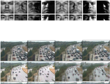
Extended Yale B dataset 1 is captured from 38 subjects and each subject has 64 front face images in different light directions and illumination conditions. All images are resized into 20 × 20 pixels.
Highway Traffic dataset 2 contains 253 video sequences of highway traffic. These sequences are labeled with three levels: 44 clips at heavy level, 45 clips at medium level and 164 clips at light level. Each video sequence has 42 to 52 frames. The video sequences are converted to gray images and each image is normalized to size 24 × 24.
1 http://vision.ucsd.edu/content/yale-face-database
2 http://www.svcl.ucsd.edu/projects/traffic/
| Methods | Num of samples | Num of clusters | D | d | r | Xi | Qi |
|---|---|---|---|---|---|---|---|
| Extended Yale B | 297 | 38 | 400 | 62 | 0.95 | G(4, 400) | G(4, 62) |
| Highway Traffic | 253 | 3 | 576 | 163 | 0.95 | G(10, 576) | G(10, 83) |
| UCF Sport | 150 | 13 | 900 | 405 | 0.95 | G(20, 900) | G(20, 405) |
(b)
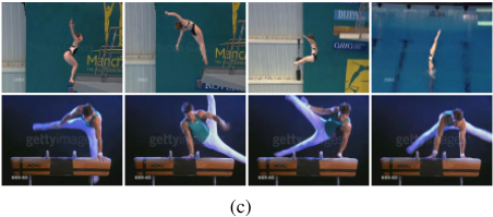
UCF sport dataset 3 includes a total of 150 sequences. The collection has a natural pool of actions with a wide range of scenes and viewpoints. There are 13 actions in this dataset. Each sequence has 22 to 144 frames. We convert these video clips into gray images and each image is resized into 30×30. Figure 2 shows some samples from these three datasets.
Parameters and evaluation
The reduced dimension d is the most important parameter for DR algorithms. Like PCA, we define d by the cumulative energy of the eigenvectors, i.e. given the remaining energy rate r (0 < r < 1), d is defined as follows,
3 http://crcv.ucf.edu/data/
where σi is the i-th largest eigenvalue of PPT , in which we stack all the Grassmann points P = [X1; ...;XN]. However, for different datasets and applications, it is difficult to set a proper r uniformly. For simplification and fairness, here we set r = 0.95 in all our experiments.
The performance of different algorithms is evaluated by Accuracy (ACC) and we also add Normalized Mutual Information (NMI) [Kvalseth, 1987] as an additional evaluation method for clustering algorithms. ACC reflects the percentage of correctly labeled samples, while NMI calculates the mutual dependence of the predicted clustering and the ground-truth partitions.
For the sake of saving space, we list all experimental parameters in Table 1. All the algorithms are coded in Matlab 2014a and implemented on an Intel Core i7-4600M 2.9GHz CPU machine with 8G RAM.
5.2 Video/Imageset Classification
We firstly evaluate the performance of GLPP on classification task, and we use K Nearest Neighbor on Grassmann manifold algorithm (GKNN) and Dictionary Learning on Grassmann manifold (GDL) [Harandi et al., 2013] as baselines,
- GKNN: KNN classifier based on the Embedding distance on high-dimensional Grassmann manifold;
- GKNN-GLPP: KNN classifier on low-dimensional Grassmann manifold obtained by the proposed method;
| Evaluation Methods | Num of Samples | ACC | ||||
|---|---|---|---|---|---|---|
| Training | Testing | GKNN | GKNN-GLPP | GDL | GDL-GLPP | |
| Dataset | Extended Yale B | |||||
| 38 sub | 221 | 76 | 94.74 | 1 | 1 | 1 |
| Dataset | Highway Traffic | |||||
| 3 sub | 192 | 60 | 70.00 | 76.67 | 65.00 | 70.00 |
| Dataset | UCF Sport | |||||
| 13 sub | 124 | 26 | 53.85 | 61.54 | 61.54 | 65.38 |
- GDL: GDL on high-dimensional Grassmann manifold;
- GDL-GLPP: GDL on low-dimensional Grassmann manifold.
Human facial recognition is one of the hottest topics in computer vision and pattern recognize area. Affected by various factors, i.e., expression, illumination conditions and light directions, algorithms based on individual faces do not achieve great experimental performance. Therefore, we test our proposed method GLPP on classic Extended Yale B dataset. We wish to inspect the proposed method on a practical application in complex environment; therefore we pick the Highway Traffic video dataset which contains various weather conditions, such as sunny, cloudy and rainy. UCF sport dataset which contains more variations on scenes and viewpoints can be used to examine the robustness of the proposed methods in noised scenarios. In our experiments, each video clip is regarded as an imageset.
To be fair, we set K = 5 for GKNN algorithm in all three experiments, and the number of training and testing samples are listed in the first two columns in Table 2, while other parameters can be found in Table 1 (i.e., D, d and r).
Experimental results for classification tasks are shown in Table 2. Obviously, the experimental accuracy of GLPPbased algorithms is at least 5 percent higher than the corresponding compared methods in most cases. We distribute it to LPP is less sensitive to outliers since LPP is derived by preserving local information. The experimental results also demonstrate that the low-dimensional Grassmann points generated by our proposed method reflect more discrimination than on the original Grassmann manifold.
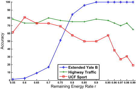
How to infer the intrinsic dimensionality from highdimensional data still is a challenging problem. The intrinsic dimensionality relies heavily on practical applications and datasets. In our method, the reduced dimensionality d is determined by the remaining energy rate r. Figure 3 shows that there exist different optimal r or d for different datasets. Extended Yale B dataset contains much rich information (e.g., face contour, texture, expression, illustration conditions and light directions) which has strong impacts on face recognition accuracy. When the reduced dimensionality d is less than the intrinsic dimensionality, the data in reduced dimensionality may lose some useful discriminative information. Therefore, the accuracy increases with larger reduced dimensionality in a certain range, e.g., the remaining energy rate r from 0.6 to
| Evaluation Methods | GKM | ACC GKM-GLPP | GKM | NMI GKM-GLPP |
|---|---|---|---|---|
| Dataset | Extended Yale B | |||
| 38 sub | 56.57 | 80.47 | 76.02 | 91.08 |
| Dataset | Highway Traffic | |||
| 3 sub | 64.43 | 73.52 | 27.13 | 38.59 |
| Dataset | UCF Sport | |||
| 13 sub | 50.00 | 57.33 | 56.54 | 62.70 |
0.95 for Extended Yale B dataset. We find the optimal value is r = 0.96. For the Traffic and UCF datasets, the simple or static backgrounds occupy main area of images. The foreground, e.g. car action and human action, is more valuable information for classification. When the optimal reduced dimensionality d is achieved at relative small r, here 0.7 and 0.8, the data in reduced dimensionality actually contain the right information for Traffic and UCF data. In other words, when the reduced dimensionality d is getting larger (> the intrinsic dimensionality), the information from the background may lead to negative influence for the accuracy.
5.3 Video/Imageset Clustering
To further verify the performance of GLPP, we apply it on clustering tasks, and select K-means on Grassmann manifold (GKM) [Turaga et al., 2011] as the compared mathod,
- GKM : K-means based on the Embedding distance on high-dimensional Grassmann manifold.
- GKM-GLPP: K-means on low-dimensional Grassmann manifold obtained by our proposed method.
Table 3 shows ACC and NMI values for all algorithms. Clearly, after drastically reducing dimensionality from D to d (see Table 1) by our proposed method, the new lowdimensional Grassmann manifold still maintain fairly higher accuracy than the original high-dimensional Grassmann manifold for all algorithms, which attests that our proposed DR scheme significantly boosts the performance of GKM.
6 Conclusion
In this paper, we extended the unsupervised LPP algorithm onto Grassmann manifold by learning a projection from the high-dimensional Grassmann manifold into the one in a relative low-dimensional with more discriminative capability, based on the strategy of embedding Grassamnn manifolds onto the space of symmetric matrices. The basic idea of LPP is to preserve the local structure of original data in the projected space. Our proposed model can be simplified as a basic eigenvalue problem for an easy solution. Compared with directly using the high-dimensional Grassmann manifold, the experimental results illustrate the effectiveness and superiority of the proposed GLPP on video/imageset classification and clustering tasks.
Acknowledgements
The research project is supported by the Australian Research Council (ARC) through the grant DP140102270 and also partially supported by National Natural Science Foundation of China under Grant No. 61390510, 61672071, 61632006, 61370119, Beijing Natural Science Foundation No. 4172003, 4162010, 4152009, Beijing Municipal Science & Technology Commission No. Z171100000517003, Project of Beijing Municipal Education Commission No. KM201610005033, Funding Project for Academic Human Resources Development in Institutions of Higher Learning Under the Jurisdiction of Beijing Municipality No.IDHT20150504 and Beijing Transportation Industry Science and Technology Project.
@inproceedings{ijcai2017p403,
  title     = {Locality Preserving Projections for Grassmann manifold},
  author    = {Wang, Boyue and Hu, Yongli and Gao, Junbin and Sun, Yanfeng and Chen, Haoran and Ali, Muhammad and Yin, Baocai},
  booktitle = {Proceedings of the Twenty-Sixth International Joint Conference on
               Artificial Intelligence, {IJCAI-17}},
  publisher = {International Joint Conferences on Artificial Intelligence Organization},
  editor    = {Carles Sierra},
  pages     = {2893--2900},
  year      = {2017},
  month     = {8},
  note      = {Main track},
  doi       = {10.24963/ijcai.2017/403},
  url       = {https://doi.org/10.24963/ijcai.2017/403},
}
TY - CPAPER TI - Locality Preserving Projections for Grassmann manifold AU - Wang, Boyue AU - Hu, Yongli AU - Gao, Junbin AU - Sun, Yanfeng AU - Chen, Haoran AU - Ali, Muhammad AU - Yin, Baocai T2 - Proceedings of the Twenty-Sixth International Joint Conference on Artificial Intelligence, IJCAI-17 PB - International Joint Conferences on Artificial Intelligence Organization PY - 2017 SP - 2893 EP - 2900 DO - 10.24963/ijcai.2017/403 UR - https://doi.org/10.24963/ijcai.2017/403 ER -Copied
Machine-readable versions of this paper, for tools and AI agents:





