
Robust Survey Aggregation with Student-t Distribution and Sparse Representation
Proceedings of the Twenty-Sixth International Joint Conference on Artificial Intelligence. Main track. Pages 2829-2835.
https://doi.org/10.24963/ijcai.2017/394
Keywords
- Machine Learning: Machine Learning
- Machine Learning: Data Mining
Abstract
Most existing survey aggregation methods assume that the sample data follow Gaussian distribution. However, these methods are sensitive to outliers, due to the thin-tailed property of the Gaussian distribution. To address this issue, we propose a robust survey aggregation method based on Student-t distribution and sparse representation. Specifically, we assume that the samples follow Student-$t$ distribution, instead of the common Gaussian distribution. Due to the Student-t distribution, our method is robust to outliers, which can be explained from both Bayesian point of view and non-Bayesian point of view. In addition, inspired by James-Stain estimator (JS) and Compressive Averaging (CAvg), we propose to sparsely represent the global mean vector by an adaptive basis comprising both data-specific basis and combined generic bases. Theoretically, we prove that JS and CAvg are special cases of our method. Extensive experiments demonstrate that our proposed method achieves significant improvement over the state-of-the-art methods on both synthetic and real datasets.
- [Aharon et al., 2006] Michal Aharon, Michael Elad, and Al- fred Bruckstein. K-svd: An algorithm for designing over- complete dictionaries for sparse representation. IEEE Transactions on Signal Processing, 54(11):4311-4322, Nov 2006.
- [Arnot et al., 2006] Chris Arnot, Peter C Boxall, and Sean B Cash. Do ethical consumers care about price? a re- vealed preference analysis of fair trade coffee purchases. Canadian Journal of Agricultural Economics/Revue cana- dienne d'agroeconomie, 54(4):555-565, 2006.
- [Bamnett and Lewis, 1994] V Bamnett and T Lewis. Out- liers in statistical data. 1994.
- [Benton et al., 2016] Adrian Benton, Michael J Paul, Braden Hancock, and Mark Dredze. Collective supervision of topic models for predicting surveys with social media. In AAAI, pages 2892-2898. AAAI Press, 2016.
- [Bock, 1975] Mary Ellen Bock. Minimax estimators of the mean of a multivariate normal distribution. The Annals of Statistics, pages 209-218, 1975.
- [Bruckstein et al., 2009] Alfred M Bruckstein, David L Donoho, and Michael Elad. From sparse solutions of systems of equations to sparse modeling of signals and images. SIAM review, 51(1):34-81, 2009.
- [Candès and Wakin, 2008] Emmanuel J Candès and Michael B Wakin. An introduction to compressive sampling. IEEE signal processing magazine, 25(2):21- 30, 2008.
- [Casella, 1985] George Casella. An introduction to empirical bayes data analysis. The American Statistician, 39(2):83- 87, 1985.
- [Chen and Huang, 2006] Peter Y Chen and Yueng-Hsiang Huang. Conducting telephone surveys. The Pschology Research Handbook: A Guide for Graduate Students and Research Assistants. London: Sage Publications, pages 210-226, 2006.
- [Dai et al., 2015] Tao Dai, Chao-Bing Song, Ji-Ping Zhang, and Shu-Tao Xia. Pmpa: A patch-based multiscale prod- ucts algorithm for image denoising. In ICIP, pages 4406- 4410. IEEE, 2015.
- [Ding and Vishwanathan, 2010] Nan Ding and SVN Vish- wanathan. t-logistic regression. In NIPS, pages 514-522, 2010.
- [Efron and Morris, 1972] Bradley Efron and Carl Morris. Limiting the risk of bayes and empirical bayes estima- torspart ii: The empirical bayes case. Journal of the Amer- ican Statistical Association, 67(337):130-139, 1972.
- [Feldman et al., 2012] Sergey Feldman, Maya Gupta, and Bela Frigyik. Multi-task averaging. In NIPS, pages 1169- 1177, 2012.
- [James and Stein, 1961] William James and Charles Stein. Estimation with quadratic loss. In Proceedings of the fourth Berkeley symposium on mathematical statistics and probability, volume 1, pages 361-379, 1961.
- [Jylänki et al., 2011] Pasi Jylänki, Jarno Vanhatalo, and Aki Vehtari. Robust gaussian process regression with a student-t likelihood. Journal of Machine Learning Re- search, 12(Nov):3227-3257, 2011.
- [Konno and Kuno, 1995] Hiroshi Konno and Takahito Kuno. Multiplicative programming problems. In Handbook of global optimization, pages 369-405. Springer, 1995.
- [Kuno et al., 1993] Takahito Kuno, Yasutoshi Yajima, and Hiroshi Konno. An outer approximation method for mini- mizing the product of several convex functions on a convex set. Journal of Global optimization, 3(3):325-335, 1993.
- [Lesage et al., 2005] Sylvain Lesage, Rémi Gribonval, Frédéric Bimbot, and Laurent Benaroya. Learning unions of orthonormal bases with thresholded singular value decomposition. In ICASSP, volume 5, pages v-293. IEEE, 2005.
- [Nair et al., 2013] Jayakrishnan Nair, Adam Wierman, and Bert Zwart. The fundamentals of heavy-tails: Properties, emergence, and identification. SIGMETRICS Perform. Eval. Rev., 41(1):387-388, June 2013.
- [O'Hagan, 1979] Anthony O'Hagan. On outlier rejection phenomena in bayes inference. Journal of the Royal Statis- tical Society. Series B (Methodological), pages 358-367, 1979.
- [Shah et al., 2014] Amar Shah, Andrew Gordon Wilson, and Zoubin Ghahramani. Student-t processes as alternatives to gaussian processes. In AISTATS, 2014.
- [Shi et al., 2016] Tianlin Shi, Forest Agostinelli, Matthew Staib, David Wipf, and Thomas Moscibroda. Improving survey aggregation with sparsely represented signals. In KDD, pages 1845-1854, NY, USA, 2016. ACM.
- [Silverman, 1986] Bernard W Silverman. Density estimation for statistics and data analysis, volume 26. CRC press, 1986.
- [Smith et al., 2015] TW Smith, PV Marsden, M Hout, and J Kim. General social surveys, 1972-2014: cumulative codebook/principal investigator, tom w, 2015.
- [Stein, 1956] Charles Stein. Inadmissibility of the usual es- timator for the mean of a multivariate normal distribution. In Proceedings of the Third Berkeley Symposium on Math- ematical Statistics and Probability, Volume 1: Contribu- tions to the Theory of Statistics, pages 197-206, Berkeley, Calif., 1956. University of California Press.
- [Tang et al., 2016] Qingtao Tang, Yisen Wang, and Shu-Tao Xia. Student-t process regression with dependent student- t noise. In ECAI 2016, The Hague, The Netherlands, volume 285, page 82. IOS Press, 2016.
- [Tropp and Gilbert, 2007] Joel A Tropp and Anna C Gilbert. Signal recovery from random measurements via orthogo- nal matching pursuit. IEEE Transactions on information theory, 53(12):4655-4666, 2007.
References were extracted automatically from the PDF and may contain errors.
Full text extracted automatically from the PDF; figures, tables and equations may differ. The PDF is the version of record.
1 Introduction
Surveys are a common way to investigate the characteristics, behaviors, or opinions of target population. Nowadays, surveys have been widely used in business [Arnot et al., 2006], data mining [Benton et al., 2016], etc. Survey-based companies (e.g., Nielsen and Kantar) earn billions of dollars per year in over 100 countries. However, conducting a survey is very expensive. For example, each short phone-call interview of a survey is charged on the order of $20-$30 in the United States, and thus even small-scale surveys can easily cost up to tens of thousands of dollars [Chen and Huang, 2006]. In addition, survey data often contain noise or outliers [Bamnett and Lewis, 1994], which have considerable effects on survey aggregation. Such high cost of conducting surveys and the issue of outliers in the survey data motivate the study of advanced survey aggregation methods that could utilize the available samples well while being robust to the outliers.
∗Equal Contribution.
The fundamental problem in aggregating survey data is to estimate the true mean response of each group of interest. A natural idea is to estimate the true means with sample means, that is, simply averaging all the samples collected within each group, which is usually referred to as sample Averaging (Avg). In fact, if the number of groups is not larger than two, Avg is uniformly better than any other method in terms of mean square error (MSE). However, if the number of groups is larger than two, it has been proved that Avg is not necessarily the best according to the Stein's paradox [Stein, 1956]. James and Stein [1961] constructed JamesStein estimator (JS) that recovers each single mean using information from all groups and outperforms Avg. Efron and Morris [1972] cast JS into an empirical Bayesian framework and showed that it is a result of maximum posterior with a prior regularization. Recently, Shi et al. [2016] proposed Compressive Averaging (CAvg) to improve JS with the compressive sensing technique [Cand`es and Wakin, 2008]. Feldman et al. [2012] proposed Multi-Task Averaging (MTAvg) by adding a penalty term to improve Avg, from the perspective of multi-task learning.
For the convenience of analysis, most existing survey aggregation methods assume that the samples are from Gaussian distribution. However, these methods do not work well on the data with outliers or heavy tails, due to the thin-tailed property of Gaussian distribution. Unfortunately, real data often exhibit heavy-tailed phenomena [Nair et al., 2013], and are common with outliers [Bamnett and Lewis, 1994]. Therefore, a robust survey aggregation method is highly demanded.
To handle the data with outliers or heavy tails, we propose a robust survey aggregation method based on Student-t distribution and sparse representation. Unlike the most existing methods based on the Gaussian distribution, we assume that the samples are from Student-t distribution, which has been proved to be a robust generalization of Gaussian distribution. Besides, inspired by JS and CAvg, we shrink the sample means to a global mean vector, and apply a sparse recovery technique to recover the global mean vector. To obtain a flexible sparse representation of the global mean vector, we design an adaptive basis which is a union of combined generic basis and data-specific basis. Theoretically, we show the robustness of our method from both Bayesian point of view and non-Bayesian point of view, and prove that both JS and CAvg are special cases of our method. Experimental results on synthetic and real data demonstrate the superiority (especially on the data with outliers) of the proposed method over the state-of-the-art methods.
2 Preliminaries
In a typical survey problem, it is common to study the characteristics of different groups, such as working time, age, or income in different regions. Specifically, assume that there are T groups in total and ni samples in group i. The quantity of interest is the true mean of certain characteristic (e.g., the mean of working hours) within each group, denoted as µi for group i (i = 1, 2, . . . , T). Samples from group i are denoted as xij (j = 1, 2, . . . , ni). The task is to estimate µ = {µi|i = 1, . . . , T} from the dataset D = {xij|i = 1, . . . , T ; j = 1, . . . , ni} as accurately as possible.
2.1 Sample Averaging
A straightforward method is to estimate the true mean µi with the sample mean ¯xi, namely, ˆµAvg i = ¯xi = 1 ni ∑ni j=1 xij. It can be proved that sample Averaging (Avg) can be interpreted as maximum likelihood estimation, given that the samples of each group are from independent and identically distributed (i.i.d.) Gaussian distribution, i.e.,
Formally, ˆµAvg i is the result of maximum likelihood estimation with the assumption (1), i.e.,
According to the analysis in [Stein, 1956], when the number of groups is one or two (i.e., T ≤ 2), Avg is uniformly better than any other method in terms of MSE. Otherwise, Avg cannot be guaranteed to be the best.
2.2 James-Stein Estimator
To improve Avg when the number of groups is larger than two, James-Stein estimator 1 (JS) was proposed in [James and Stein, 1961], which estimates the true mean of each group as
where f = 1 T ∑Ti=1 ¯xi is the global mean, γ = (T - 3)(∑Ti=1 ni σ2 i (¯xi - f)2)-1 , and (·)+ = max(0, ·); σ2 i is the variance of group i (usually unknown in real data) and is replaced by a standard unbiased estimate. Note that unlike Avg, JS shrinks the sample means ¯xi's towards the global mean f. Efron and Morris [1972] proved that JS is the maximum posterior estimation with the Gaussian sample assumption (1) and the following assumption,
where A is the variance of the prior. Compared with Avg, JS adds the prior assumption (4) with respect to µi.
1 The original James-Stein estimator has many variants. Following [Feldman et al., 2012; Shi et al., 2016], in this paper, we use the positive part James-Stein estimator with independent unequal variances [Bock, 1975; Casella, 1985].
2.3 Compressive Averaging
It has been shown in [Shi et al., 2016] that JS performs poorly when the distance between ¯xi and f becomes large (see the example in [Shi et al., 2016], Section 3.1). To overcome this drawback, Shi et al. [2016] proposed an improvement of JS based on compressive sensing, named Compressive Averaging (CAvg). Specifically, CAvg assumes
where {f1, f2, . . . , fT }, denoted as f , is the global mean vector, which is assumed to be sparsely represented by a given basis. Besides, CAvg assumes that the sample means ¯xi's followGaussian distribution, i.e.,
At the first glance, the assumptions (6) and (1) seem different ((1) can lead to (6) directly, but not vice versa). However, these two assumptions actually make no difference for maximum posterior (to estimate µi) and maximum marginal likelihood (to estimate parameters f and A), which will be explained next separately. For the maximum posterior, its result in CAvg is (see (11) in [Shi et al., 2016])
which is also the result of maximum posterior based on the assumptions (1) and (5), i.e.,
For the maximum marginal likelihood, we will show that the assumptions (6) and (1) have no difference in Section 4. Since the assumptions (6) and (1) have no difference for both maximum posterior and maximum marginal likelihood, we claim that CAvg is consistent with the Gaussian sample assumption (1).
2.4 Multi-Task Averaging
The idea of using information from all groups to improve the estimate of some quantities of a single group falls into the realm of multi-task learning in artificial intelligence and machine learning community. From this perspective, Feldman et al. [2012] proposed Multi-Task Averaging (MTAvg), which estimates µi (i = 1, 2, . . . , T ) by minimizing
where S is a pairwise task similarity matrix. MTAvg can be interpreted as estimating the means of T Gaussians with an intrinsic Gaussian Markov random field prior [Feldman et al., 2012]. Note that the square loss in MTAvg corresponds to the Gaussian sample assumption (1).
3 Robust Survey Aggregation
3.1 Motivation
As discussed in Section 2, all the above methods, including Avg, JS, CAvg, and MTAvg, share the common Gaussian sample assumption (1) explicitly or implicitly. Based on such assumption, the inference is relatively easy. However, this assumption results in severe problems in practice. I) Real data often exhibit heavy-tailed phenomena, which are beyond the Gaussian distribution. Fig. 1(a) shows the heavy-tailed phenomenon in real dataset Hrs1 from the yearly General Social Survey [Smith et al., 2015]. The density of Hrs1 is estimated by kernel density estimation [Silverman, 1986]. Student-t distribution and Gaussian distribution fit the data respectively with the method of moments. It can be observed that the Student-t fitting density is much closer to the estimated density of Hrs1 than the Gaussian fitting density, because the real distribution has heavy tails; II) real data often contain noise or outliers, which deteriorate the performance of Gaussian based methods. The effect of outliers can be seen in Table 1 (the experimental details will be introduced in Section 5), from which we can observe that MSEs of Avg, JS, CAvg, and MTAvg increase a lot (all over 60%) when 2% of the data are contaminated with outliers.
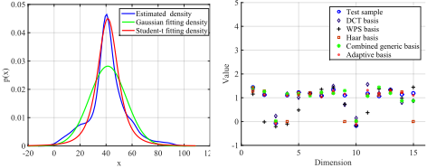
(a) Density fitting for Hrs1
(b) Signal sparse representation
Figure 1: (a) Heavy-tailed phenomenon in the real data Hrs1. (b) Sparse recovery results by OMP with different bases.
The issues caused by the Gaussian sample assumption (1) motivate us to design a robust survey aggregation method.
3.2 Derivation of Robust Survey Aggregation
To handle the survey data with outliers or heavy tails, we propose Robust Averaging (RAvg), in which the samples are assumed to follow Student-t distribution, i.e.,
where ν is degrees of freedom; σ2 = {σ2 i |i = 1, . . . , T} is the set of scale parameters, which can be replaced by a standard unbiased estimate, similarly as in JS and CAvg.
The reasons for using the Student-t sample assumption (10) instead of the Gaussian sample assumption (1) are as follows: I) Student-t sample assumption (10) is a natural generalization of Gaussian sample assumption (1). When degrees of freedom ν approaches +∞, Student-t sample assumption (10) reduces to Gaussian sample assumption (1). II) Student-t distribution, which is a heavy-tailed distribution, has been proved to be a robust alternative to Gaussian distribution in [O'Hagan, 1979; Shah et al., 2014;
Tang et al., 2016], from Bayesian point of view. Besides, the robustness from Student-t sample assumption (10) can be also shown from non-Bayesian view, which will be discussed in detail in Section 4.
Therefore, we expect our method based on the Student-t sample assumption (10) is more robust to outliers and can be applied to more types of data.
Similar to CAvg, we also assume the true means
where fi encodes a flexible prior about µi, and A controls how strong the prior is.
Based on the assumptions (10) and (11), we minimize the negative log marginal likelihood of RAvg to learn the parameters A, ν, f = {fi|i = 1, . . . , T}, followed by estimating the target µi via minimum negative log posterior.
The marginal likelihood can be derived as follows based on the assumptions (10) and (11),
Since (12) is analytically intractable, we rely on Laplace approximation [Jyl¨anki et al., 2011] for approximate inference. Particularly, we use a second order Taylor expansion of Ψ(µ) locally around ˆµ=argµmaxΨ(µ), and obtain Ψ(µ) ≃ Ψ( ˆµ) - 1 2 (µ - ˆµ)⊤Σ-1 (µ - ˆµ). Thus, an approximation, q(D|f , A, ν), to the marginal likelihood is
where Σ-1 is the negative Hessian matrix of Ψ(µ) at ˆµ. Particularly, Σ-1 is a diagonal matrix with
Based on the following fact,
an approximation to the negative log marginal likelihood is
The details of learning the parameters A, ν, and f by minimizing (13) will be introduced in Section 3.3. Once the parameters A, ν, and f are learned, the estimation of µi can be obtained by minimum negative log posterior of RAvg, i.e., minimizing the following objective:
The exponent of (14) is a product of positive convex functions, and thus minimizing the exponent of (14) (equivalent to minimizing (14)) belongs to the convex multiplicative programming [Konno and Kuno, 1995], which can be efficiently obtained by the method in [Kuno et al., 1993] (also refer to the convex multiplicative programming in robust logistic regression [Ding and Vishwanathan, 2010]).
3.3 Parameter Learning
When minimizing the negative log marginal likelihood in (13) to learn the parameters A, ν, f , we need to restrict f by adding some assumptions. Inspired by [Shi et al., 2016], we assume that f can be sparsely represented by a given basis Φ = {φ1, . . . , φK} with φi ∈ RT×1 , i.e., f = Φα = ∑Ki=1 αiφi, where α = {α1, . . . , αK} is a sparse coefficient vector with ||α||0 ≤ k ≪ K, in which ||α||0 is ℓ0 norm that counts the non-zero elements in α.
Then, we solve the minimum negative log marginal likelihood in (13) by updating two sets of parameters {A, ν} and α alternatively until the objective of (13) converges.
- Fix α, solve for A, ν. (13) is differentiable with respect to A, ν, and thus we can use gradient based optimization methods. An alternative approach is to estimate a rough range of A, ν and search the optimum with linear search algorithm, considering that A, ν are scalars.
- Fix A, ν, solve for α. The optimization problem is
This problem resembles the sparse recovery formulation in compressive sensing [Cand`es and Wakin, 2008], which can be solved by classical algorithms, such as Orthogonal Matching Pursuit (OMP) [Tropp and Gilbert, 2007]. For simplicity and efficiency, we adopt the linear search algorithm to solve for A, ν, and use OMP to solve for α.
3.4 Adaptive Basis
As discussed above, the global mean vector f can be sparsely represented by a given basis Φ. Nonetheless, it is non-trivial to choose the basis, since different types of signals typically have different characteristics [Bruckstein et al., 2009; Dai et al., 2015]. In CAvg, Shi et al. [2016] empirically used the single Daubechies least-asymmetric wavelet packet (WPS), which cannot always lead to sparse solutions. Taking Fig. 1(b) for example, the WPS basis performs poorly on the electricity consumption data ("elec35 nor", a built-in dataset in Matlab).
The poor performance of WPS motivates us to design a more generalizable basis that can be used for a wide range of signals of interest. A straightforward idea is to unify different types of generic bases (e.g., discrete cosine transform (DCT) basis, WPS basis, Haar basis) in a combined representation [Lesage et al., 2005], denoted as combined generic basis ˜Φc,
where Φj ∈ RT×Kj , j = 1, 2, . . . ,M are different types of generic bases. Compared with the single basis, the major advantage of the combined generic basis ˜Φc is the relative simplicity of the pursuit algorithm and better generalization ability to different signals. However, combined generic basis ˜Φc generally cannot work well on an arbitrary unseen family of signals of interest, where an adaptive data-specific basis usually performs better [Bruckstein et al., 2009].
To obtain a data-specific basis, K-SVD [Aharon et al., 2006] algorithm has been widely used in sparse representation. When applying K-SVD algorithm to the survey data, the problem is that the sample size is usually small for KSVD. To address this issue, denoting the data-specific basis learned by K-SVD algorithm as ˜Φl, we cascade combined generic basis ˜Φc (a prior) and data-specific basis ˜Φl as
which is our final adaptive basis.
To demonstrate the effectiveness of our adaptive basis, we randomly select 50 samples for training and 1 sample for testing, from the electricity consumption data. The test sample and sparse recovery results produced by OMP with various bases, namely DCT basis, WPS basis, Haar basis, combined generic basis (union of DCT, WPS and Haar basis), and our adaptive basis are shown in Fig. 1(b), from which we can observe that our adaptive basis produces the best results while the generic bases fail to achieve satisfactory results.
4 Theoretical Analysis
In this section, we prove that CAvg and JS are special cases of our RAvg method, and show that our RAvg method is more robust to outliers than Avg, JS, CAvg, and MTAvg from the view of loss and penalty.
Theorem 1 CAvg is a special case of RAvg with ν → +∞ and WPS basis.
Proof. When ν → +∞, the minimum negative log posterior of RAvg (i.e., (14)) converges to that of CAvg (i.e., (8)). Then, as long as the parameters A, f in the posterior are also identical, CAvg and RAvg will generate the same estimation for µi. As the parameters A, f are learned by minimum negative log marginal likelihood, we only need to prove that their minimum negative marginal likelihoods are equivalent when using the same WPS basis.
With ν → +∞, it is not hard to prove that ˆµ and Σ-1 in the approximate procedure have the forms
By substituting ˆµi and Σii in (16) into (13) and with simplifications, we can obtain
Recall that σ2 i is replaced by a standard unbiased estimate, with ν → +∞, we can obtain the following two equations:
By substituting (18) and (19) into (17) and omitting the constant, we obtain
which is exactly the same as the minimum negative log marginal likelihood of CAvg (see [Shi et al., 2016], (10)), i.e., minimum negative marginal likelihood of RAvg is equivalent to that of CAvg. So we complete the proof here. □
With (18) and (19), it is easy to prove that CAvg is consistent with the Gaussian sample assumption implicitly, as mentioned in Section 2.3. Specifically, for CAvg, when replacing the assumption (6) with the assumption (1), the minimum negative log marginal likelihood of CAvg is equivalent to (20). Besides, as discussed in Section 2.3, the assumptions (6) and (1) also make no difference for maximum posterior. Thus, CAvg is consistent with the Gaussian sample assumption (1) implicitly.
Theorem 2 JS is a special case of RAvg with ν → +∞, the equal elements in f , and identical parameter estimation.
Proof. When ν → +∞, the Student-t sample assumption (10) reduces to the Gaussian sample assumption (1). When the elements in f of RAvg, i.e., f1, . . . , fT , are equal, JS and RAvg have the same assumptions. Furthermore, when the parameters A and f of RAvg are estimated using the method in JS (see [Efron and Morris, 1972; Casella, 1985]), RAvg will produce the same estimation as JS. □
Proposition 1 From the view of loss and penalty, RAvg is more robust than Avg, JS, CAvg, and MTAvg.
From Bayesian view, we know that RAvg is more robust than those Gaussian based methods (i.e., Avg, JS, CAvg, and MTAvg) due to the Student-t sample assumption (10), as discussed in Section 3.2. In fact, from non-Bayesian view, the robustness of RAvg can also be explained as follows. The optimization objectives of all the methods for µi, Avg (2), JS
((8) with all fi's equal), CAvg (8), MTAvg (9), and RAvg (14) can be interpreted as a loss term plus a penalty (for Avg, the penalty is 0). We can see that for Avg, JS, CAvg and MTAvg, the loss function is square loss. In contrast, the loss function of RAvg is a log-square loss, which is much more robust.
5 Experiments
In this section, we conduct comprehensive experiments on both synthetic and real datasets. Our baselines include Avg, JS, MTAvg, and CAvg. For fair comparison, OMP is also used to calculate α in CAvg and k is set as 3 for both RAvg and CAvg, following [Shi et al., 2016]. The evaluation metric is the mean square error (MSE) between the true mean and the estimated mean of each group. Note that the true means are known for synthetic data, but unknown for real data. Following [Shi et al., 2016], the true means are replaced by the sample means when 100% of the data are used.
5.1 Datasets
The datasets for the experiments include
- Synthetic Data A. This dataset is created according to the generative procedure in [Shi et al., 2016]. The sample assumption is Gaussian, in which there are 10 groups with 100 samples in each group.
- GSS. General Social Survey (GSS) is a well-known public survey dataset [Smith et al., 2015]. We take out the variables Age, Hrs1, Paedu, and Spedu from GSS. Age means the age of the respondent, with 30 groups, each of which contains 1372 ∼ 4492 samples. Hrs1 refers to the number of working hours the respondent had last week, with 29 groups, each of which contains 741 ∼ 2739 samples. Paedu stands for the highest school year completed by the respondent's father, with 30 groups, each of which contains 1051 ∼ 2258 samples. Spedu denotes the highest school year completed by the respondent's spouse, with 30 groups, each of which contains 721 ∼ 1458 samples.
5.2 Performance on Synthetic and Real Datasets
| Avg | JS | MTAvg | CAvg | RAvg | |
|---|---|---|---|---|---|
| Original data | 2.575 | 2.201 | 2.131 | 2.106 | 2.013 |
| With 2% outliers | 4.192 | 3.656 | 3.598 | 3.603 | 2.372 |
| Increased MSE | 1.617 | 1.455 | 1.467 | 1.503 | 0.359 |
The experimental results on the Synthetic Data A are reported in Table 1, from which we observe that RAvg has comparable result with CAvg even though the samples are from Gaussian distribution. The underlying reason is that the Student-t sample assumption includes the Gaussian sample assumption as a special case and our basis is adaptive. Moreover, when 2% of the samples are contaminated with outliers, RAvg is statistically better than other methods with 95% confidence.
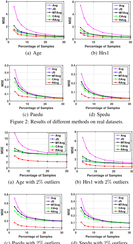
For the real datasets, we randomly select some samples from each dataset and use these samples to estimate the true means (the means when 100% of the data are used). We vary the sampling percentage from 3% to 30%, run each method for 30 runs, and compute the average MSE of 30 runs. The results of different methods on the real datasets are plotted in Fig. 2, from which we can observe that our RAvg method outperforms all the baselines for all percentages of samples.
In the experiments, RAvg takes more time than baselines (Specifically, 3 ∼ 5 times more than CAvg). However, the sample size is usually small, since each sample point is expensive (see Introduction). Thus, time complexity is not the key issue for survey aggregation.
5.3 Robustness to Outliers
The robustness of RAvg has been shown on the synthetic data, as demonstrated in Table 1. In order to evaluate the robustness on real datasets, 2% of the samples are contaminated with outliers and the results of all methods are reported in Fig. 3. Comparing Fig. 2 and Fig. 3, we can see that once the data are contaminated with outliers, MSEs of Avg, JS, MTAvg, and CAvg increase significantly while RAvg remains steady and achieves much better performance than other methods, which demonstrates the robustness of RAvg on the real datasets.
5.4 Component Analysis
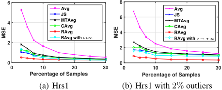
To investigate the individual contribution of the Student-t sample assumption and the adaptive basis in our proposed RAvg method, we introduce RAvg with ν → +∞ (in practice, ν is fixed to 100), which reduces to CAvg except using adaptive basis, based on Theorem 1. Therefore, the gap between RAvg with ν → +∞ and RAvg is caused by the Student-t sample assumption, and the gap between RAvg with ν → +∞ and CAvg is the contribution of the adaptive basis. Taking the Hrs1 dataset as an example, Fig. 4 shows the results, where we can observe that the adaptive basis reduces the MSE, and the Student-t sample assumption further reduces the MSE, since the density of Hrs1 has heavy tails, as illustrated in Fig. 1(a). It is worth noting that the contribution of the Student-t assumption is more significant when the data are contaminated with outliers, as shown in Fig. 4(b).
6 Conclusion
In this paper, we propose a robust survey aggregation method, RAvg, based on Student-t sample assumption and sparse representation. In particular, due to the Student-t sample assumption, our method is robust to outliers, which is analyzed in detail from Bayesian point of view and loss-penalty point of view. For a better sparse representation of the global mean vector, we design a simple yet effective adaptive basis, which further improves the performance. Theoretically, we have proved that JS and CAvg are special cases of our method. Extensive experiments have demonstrated that our method significantly outperforms the state-of-the-art methods, especially in the presence of outliers.
Acknowledgments
This work is supported by the National Natural Science Foundation of China under grant Nos. 61371078, 61375054, and the R&D Program of Shenzhen under grant Nos. JCYJ20140509172959977, JSGG20150512162853495, ZDSYS20140509172959989, JCYJ20160331184440545. This work is partially supported by NTU-SCSE Grant 2016-2017 and NTU-SUG (CoE) Grant 2016-2018.
@inproceedings{ijcai2017p394,
  title     = {Robust Survey Aggregation with Student-t Distribution and Sparse Representation},
  author    = {Tang, Qingtao and Dai, Tao and Niu, Li and Wang, Yisen and Xia, Shu-Tao and Cai, Jianfei},
  booktitle = {Proceedings of the Twenty-Sixth International Joint Conference on
               Artificial Intelligence, {IJCAI-17}},
  publisher = {International Joint Conferences on Artificial Intelligence Organization},
  editor    = {Carles Sierra},
  pages     = {2829--2835},
  year      = {2017},
  month     = {8},
  note      = {Main track},
  doi       = {10.24963/ijcai.2017/394},
  url       = {https://doi.org/10.24963/ijcai.2017/394},
}
TY - CPAPER TI - Robust Survey Aggregation with Student-t Distribution and Sparse Representation AU - Tang, Qingtao AU - Dai, Tao AU - Niu, Li AU - Wang, Yisen AU - Xia, Shu-Tao AU - Cai, Jianfei T2 - Proceedings of the Twenty-Sixth International Joint Conference on Artificial Intelligence, IJCAI-17 PB - International Joint Conferences on Artificial Intelligence Organization PY - 2017 SP - 2829 EP - 2835 DO - 10.24963/ijcai.2017/394 UR - https://doi.org/10.24963/ijcai.2017/394 ER -Copied
Machine-readable versions of this paper, for tools and AI agents:





