
Fast Sparse Gaussian Markov Random Fields Learning Based on Cholesky Factorization
Proceedings of the Twenty-Sixth International Joint Conference on Artificial Intelligence. Main track. Pages 2758-2764.
https://doi.org/10.24963/ijcai.2017/384
Keywords
- Machine Learning: Learning Graphical Models
- Multidisciplinary Topics and Applications: Computational Biology and e-Health
- Machine Learning: Unsupervised Learning
Abstract
Learning the sparse Gaussian Markov Random Field, or conversely, estimating the sparse inverse covariance matrix is an approach to uncover the underlying dependency structure in data. Most of the current methods solve the problem by optimizing the maximum likelihood objective with a Laplace prior L1 on entries of a precision matrix. We propose a novel objective with a regularization term which penalizes an approximate product of the Cholesky decomposed precision matrix. This new reparametrization of the penalty term allows efficient coordinate descent optimization, which in synergy with an active set approach results in a very fast and efficient method for learning the sparse inverse covariance matrix. We evaluated the speed and solution quality of the newly proposed SCHL method on problems consisting of up to 24,840 variables. Our approach was several times faster than three state-of-the-art approaches. We also demonstrate that SCHL can be used to discover interpretable networks, by applying it to a high impact problem from the health informatics domain.
- [Banerjee et al., 2008] Onureena Banerjee, Laurent El Ghaoui, and Alexandre d'Aspremont. Model se- lection through sparse maximum likelihood estimation for multivariate gaussian or binary data. The Journal of Machine Learning Research, 9:485-516, 2008.
- [Banerjee et al., 2014] Sudipto Banerjee, Bradley P Carlin, and Alan E Gelfand. Hierarchical modeling and analysis for spatial data. Crc Press, 2014.
- [Boyd and Vandenberghe, 2004] Stephen Boyd and Lieven Vandenberghe. Convex optimization. Cambridge, 2004.
- [Dahl et al., 2008] Joachim Dahl, Lieven Vandenberghe, and Vwani Roychowdhury. Covariance selection for non- chordal graphs via chordal embedding. Optimization Methods & Software, 23(4):501-520, 2008.
- [Dempster, 1972] Arthur P Dempster. Covariance selection. Biometrics, pages 157-175, 1972.
- [Dobra et al., 2004] Adrian Dobra, Chris Hans, Beatrix Jones, Joseph Nevins, Guang Yao, and Mike West. Sparse graphical models for exploring gene expression data. Jour- nal of Multivariate Analysis, 90(1):196-212, 2004.
- [Duchi et al., 2008] John Duchi, Stephen Gould, Daphne Koller, et al. Projected subgradient methods for learn- ing sparse gaussians. In Proceedings of the Twenty-Fourth Conference on Uncertainty in Artificial Intelligence, 2008.
- [Friedman et al., 2008] Jerome Friedman, Trevor Hastie, and Robert Tibshirani. Sparse inverse covariance estima- tion with the graphical lasso. Biostatistics, 9(3), 2008.
- [Hsieh et al., 2011] Cho-Jui Hsieh, Inderjit S Dhillon, Pradeep K Ravikumar, and Mátyás A Sustik. Sparse in- verse covariance matrix estimation using quadratic ap- proximation. In Advances in Neural Information Process- ing Systems, pages 2330-2338, 2011.
- [Hsieh et al., 2013] Cho-Jui Hsieh, Mátyás A Sustik, Inder- jit S Dhillon, Pradeep K Ravikumar, and Russell Poldrack. Big & quic: Sparse inverse covariance estimation for a million variables. In Advances in Neural Information Pro- cessing Systems, pages 3165-3173, 2013.
- [Huang et al., 2006] Jianhua Z Huang, Naiping Liu, Mohsen Pourahmadi, and Linxu Liu. Covariance matrix se- lection and estimation via penalised normal likelihood. Biometrika, 93(1):85-98, 2006.
- [Koller and Friedman, 2009] Daphne Koller and Nir Fried- man. Probabilistic graphical models: principles and tech- niques. MIT press, 2009.
- [Lauritzen, 1996] Steffen L Lauritzen. Graphical models. Clarendon Press, 1996.
- [Li, 2012] Stan Z Li. Markov random field modeling in com- puter vision. Springer Science & Business Media, 2012.
- [Meinshausen and Bühlmann, 2006] Nicolai Meinshausen and Peter Bühlmann. High-dimensional graphs and variable selection with the lasso. The annals of statistics, 34(3):1436-1462, 2006.
- [Parnell et al., 2013] Grant P Parnell, Benjamin M Tang, Marek Nalos, Nicola J Armstrong, Stephen J Huang, David R Booth, and Anthony S McLean. Identifying key regulatory genes in the whole blood of septic pa- tients to monitor underlying immune dysfunctions. Shock, 40(3):166-174, 2013.
- [Rolfs et al., 2012] Benjamin Rolfs, Bala Rajaratnam, Do- minique Guillot, Ian Wong, and Arian Maleki. Iterative thresholding algorithm for sparse inverse covariance esti- mation. In Advances in Neural Information Processing Systems, pages 1574-1582, 2012.
- [Scheinberg and Rish, 2010] Katya Scheinberg and Irina Rish. Learning sparse gaussian markov networks using a greedy coordinate ascent approach. In Machine Learning and Knowledge Discovery in Databases, pages 196-212. Springer, 2010.
- [Stojkovic et al., 2016a] Ivan Stojkovic, Mohamed F. Ghal- wash, Xi Hang Cao, and Zoran Obradovic. Effective- ness of Multiple Blood-Cleansing Interventions in Sepsis, Characterized in Rats. Scientific Reports, 6(24719):1-11, 2016.
- [Stojkovic et al., 2016b] Ivan Stojkovic, Vladisav Jelisavcic, Veljko Milutinovic, and Zoran Obradovic. Distance based modeling of interactions in structured regression. In Pro- cedeengs of the 25th International Joint Conference on Ar- tificial Intelligence (IJCAI-16), pages 2032-2038, 2016. IJCAI
- [Stuart et al., 2003] Joshua M Stuart, Eran Segal, Daphne Koller, and Stuart K Kim. A gene-coexpression network for global discovery of conserved genetic modules. Sci- ence, 302(5643):249-255, 2003.
- [Tibshirani, 1996] Robert Tibshirani. Regression shrinkage and selection via the lasso. Journal of the Royal Statistical Society. Series B (Methodological), pages 267-288, 1996.
- [Treister and Turek, 2014] Eran Treister and Javier Turek. A block-coordinate descent approach for large-scale sparse inverse covariance estimation. In Advances in Neural In- formation Processing Systems, pages 927-935, 2014.
- [Wang et al., 2016] Min Wang, Jingjun Yan, Xingxing He, Qiang Zhong, Chengye Zhan, and Shusheng Li. Can- didate genes and pathogenesis investigation for sepsis- related acute respiratory distress syndrome based on gene expression profile. Biological research, 49(1):1-9, 2016.
- [Wen et al., 2012] Zaiwen Wen, Wotao Yin, Hongchao Zhang, and Donald Goldfarb. On the convergence of an active-set method for l1 minimization. Optimization Meth- ods and Software, 27(6):1127-1146, 2012.
- [Wytock and Kolter, 2013] Matt Wytock and Zico Kolter. Sparse gaussian conditional random fields: Algorithms, theory, and application to energy forecasting. In Interna- tional conference on machine learning, pages 1265-1273, 2013.
- [Yuan and Lin, 2007] Ming Yuan and Yi Lin. Model se- lection and estimation in the gaussian graphical model. Biometrika, 94(1):19-35, 2007.
References were extracted automatically from the PDF and may contain errors.
Full text extracted automatically from the PDF; figures, tables and equations may differ. The PDF is the version of record.
1 Introduction
Markov Random Fields, or undirected networks, are a prominent class of probabilistic graphical models that can characterize the dependency structure among a set of random variables [Koller and Friedman, 2009]. As inference in these models is generally intractable, a Gaussian assumption is often assumed to make it tractable and computationally efficient, giving rise to Gaussian Markov Random Field (GMRF) models. Commonly, the observations of many multivariable processes of interest are effectively approximated by a multivariate normal distribution, allowing reliable GMRF learning.
Although the Gaussian assumption of the model allows for efficient inference and learning, its utility also depends on the properties of the underlying connectivity structure. Sparsity in the model parametrization is well aligned with the desirable property of the model parsimony (Occam's razor). Sparsity also reduces the tendency of overfitting, and increases the interpretability of the model by exposing essential relations between the variables. Therefore, enforcing sparsity when learning GMRFs is an attractive way to discover the underlying structure in the data, which makes sparse GMRF a handy tool applicable in various domains with highdimensional data, including bio-medical [Dobra et al., 2004], spatial [Banerjee et al., 2014] and computer vision [Li, 2012].
∗These two authors contributed equally
Learning a GMRF model is shown to be equivalent to reconstructing the inverse covariance matrix (a.k.a precision) from the data. The precision matrix essentially carries information about conditional dependence between the variables, or equivalently of the graph connectivity patterns. There exist several methods developed to solve the problem of sparse inverse covariance estimation which we briefly introduce in section II. In that body of work, special attention is devoted to the computational efficiency of methods. With an ever increasing size and dimensionality of available data, there is a necessity for even faster and more efficient algorithms.
We propose a novel method for fast learning of sparse GMRFs from high-dimensional data, that relies on Cholesky decomposition. In section III, we introduce a new sparsity inducing regularization term, based on L1 norm, that penalizes an approximate product of two Cholesky factors. The resulting objective function is convex and can be efficiently optimized by the coordinate descent based SCHL algorithm. Further substantial speedup is achieved by developing an active set approach, which reduces unnecessary computations by focusing only on a subset of active parameters. In section IV, we compare the proposed SCHL method against three stateof-the-art approaches, on synthetic problems of varying sizes. The empirical evaluations suggest that our method is several times faster than the best of the competing approaches. The results also provide evidence that obtained solutions of all evaluated methods have comparable quality. We also provide analysis of the applicability of our SCHL method for discovering the meaningful structures in high impact applications involving gene expression levels in septic patients.
2 RelatedWork
Sparse inverse covariance learning was first introduced as a problem to find the maximum likelihood model with a minimal number of nonzero parameters (the L0 norm penal) [Dempster, 1972]. However, this combinatorial optimization problem quickly becomes intractable with an increase in the number of variables. Initial approaches to address this challenge were based on a greedy search in a space of possible graphs [Lauritzen, 1996], which did not scale well due to the necessity of calculating a maximum likelihood in each iteration, and were also inapplicable in cases where dimensionality was greater than the number of samples.
Often, the number of samples is smaller than the number of measured variables, so the necessity for an applicable solution yielded a different approach to learning the sparse precision matrix from the data. The intractable problem with L0 norm was approximated by a convenient convex formulation with L1 norm, which also enforces a degree of sparsity in the solution. The first method that utilized L1 norm was the neighborhood selection approach [Meinshausen and B¨uhlmann, 2006], which selected connected variables by solving a number of decoupled LASSO [Tibshirani, 1996] problems. Although the approach is not directly solving the L1 regularized maximum likelihood problem, it can be seen as a simple approximation of that problem.
Several approaches followed [Yuan and Lin, 2007; Dahl et al., 2008; Banerjee et al., 2008], that were exactly solving the L1 penalized maximum likelihood problem using convex optimization tools [Boyd and Vandenberghe, 2004]. other methods were proposed to provide further improvement. Graphical LASSO [Friedman et al., 2008] improved the computational efficiency of learning the sparse precision matrix by proposing a faster optimization based on a coordinate descent algorithm. In [Duchi et al., 2008], authors proposed a fast projected gradient method, which can solve even more general types of problems with block-sparsity. While previously mentioned methods optimized the dual of the problem, the SINCO algorithm [Scheinberg and Rish, 2010] solved the direct problem by utilizing a greedy coordinate ascent. A GISTA approach [Rolfs et al., 2012], based on the proximal gradient method, has attractive theoretical guarantees regarding the error bounds and linear convergence rates.
All the algorithms mentioned so far utilize only the first order gradient information, which limits their convergence to linear at best. The QUIC approach [Hsieh et al., 2011] proposed the use of a second order information based on Newton's method, in order to provide superlinear convergence and a substantial increase in computational efficiency. The algorithm was subsequently improved into BIG & QUIC [Hsieh et al., 2013] by adopting the block coordinate descent method, where blocks are obtained by clustering. Block-wise optimization helped reduce the memory requirements, as it needs only part of the precision matrix to be stored, which allowed scaling to large problems. BCDIC [Treister and Turek, 2014] is another memory efficient algorithm for large-scale inverse covariance learning based on block coordinate descent.
3 Method
We propose a novel SCHL method for fast learning of sparse GMRF, by decomposing the precision matrix into a product of two Cholesky factors, and imposing L1 penalty on the approximation of that product. Our approach is related but distinct from the CSEPNL approach that directly penalizes the entries of a Cholesky factor itself [Huang et al., 2006].
3.1 Problem Setup
The sparse inverse covariance Σ-1 estimation problem is defined as minimizing the negative log-likelihood of a Gaussian
subject to positive definite constraint ytΣ-1 y > 0, ∀y ∈ IRn .
3.2 SCHLMethod
The main computational burden in finding the optimal solution of the problem (1) comes from calculating the log|Σ-1 | term, which in a naive implementation would require O(N 3 ) steps. We propose different parametrization, which enables calculating the log|Σ-1 | in a more efficient manner.
Recent efficient approaches are based on the coordinate descent optimization and in combination with an active set method are shown to be applicable to large-scale problems [Hsieh et al., 2013]. However, most models based on the active set method need to evaluate the active condition for each variable every iteration, which is prohibitively expensive for big data. We propose a different sparsity penal, that enables us to determine the active set as a preprocessing step, and effectively avoid iterating over all variables on each sweep of coordinate descent.
We start the analysis from Cholesky reparametrization of the problem (1). Since the precision matrix is positive definite, it can be decomposed into Cholesky factors: Σ-1 = LLT where L is a lower-triangular matrix with positive diagonal entries. It can be easily shown that in such parametrization of problem (1), the positive definite constraint is encoded into a simpler constraint Lii > 0. Also, we note several other benefits, which we build our approach upon: 1) For a sufficiently sparse Cholesky matrix L, LLT will also be sparse; 2) Cholesky factors can be efficiently used to calculate the inverse. By having Cholesky factors always available at no additional cost, expensive matrix inversion operations can be done more efficiently. Besides these benefits, using a Cholesky parametrization of objective (1) also has some downsides, as regularizing the precision matrix becomes increasingly difficult to optimize in terms of new parameters. In order to solve this problem, we introduce a different penalty term based on the relaxation of the original objective.
In order to derive update equations, we follow the standard approach to separate problem (1) into differentiable g(L) and non-differentiable h(L) parts:
First, we analyze the differentiable part, expressed in the introduced reparametrization:
The following can be easily shown using the identity det(LLT ) = ∏Ni=1 L2ii :
In order to minimize the objective we compute derivatives ∂g ∂Lij . There are two separate cases: i = j, and i ̸= j.
For off-diagonal elements (i ̸= j):
where S = yyT is the empirical covariance matrix.
Next, we compute diagonal derivatives:
Now when we have expressions for derivatives, the differential part (3) can be optimized using coordinate descent by finding zeros of equations (5) (linear) and (6) (quadratic):
The second solution to the quadratic equation is always discarded, since Lii must be positive in order for the Σ-1 matrix to be positive definite. By looking at the update equations (7) and (8) we notice that if L is sparse with space complexity O(Sactive), calculating updates will also have O(Sactive) time complexity.
Sparsity Through L1 Regularization
In order to learn structure from the data, we rely on the sparsity inducing L1 norm. Previous work [Yuan and Lin, 2007; Banerjee et al., 2008; Friedman et al., 2008] relies on applying the L1 penalty on the elements of a precision matrix. However, since our method relies on Cholesky parametrization, and the precision matrix is a function of parameters in our setting, handling the L1 penalty term is not straightforward. To derive appropriate subgradient equations we start from the ordinary penalty term:
where ||LLT ||1 is the sum of absolute entries of the precision matrix:
None of the terms under L1 norm in eq. (10) are convex, so optimizing the global objective (1) is hard, since none of the standard convex optimization tools can be used. In order to solve this, we propose a relaxation of the penalty term:
This relaxed penalty acts slightly different than the original L1 penalty on the precision matrix. However, for sufficiently sparse problems, it can be shown that they behave similarly since they both induce sparsity on parameters L of optimization and because sufficiently sparse Cholesky factors lead to a sparse precision matrix. In Appendix A we outline the proof that this relaxed penalty (11) is convex, for suitably selected parameters λij. Without loss of generalization, we will assume that the λij are all identical in the further text.
The new objective, with penal defined in (11), can be optimized using the coordinate descent method. Now, let's observe the sub-gradient of h(L), and its (m, n) component:
where Amn is the value of the derivative over variables Lmn where it exists. We start fromAmn:
Finally, we get:
Expression for the (m, n) component of the sub-gradient of h(L) is therefore:
The sub-gradient of the whole optimization function now can be written as:
where Z = ∑k LkjSki and i ̸= j. Therefore, if following condition is satisfied:
parameter Lij will be zero. For the sub-gradient ∇l(L)ii the following equation holds (using the fact that Lii must be positive, therefore always larger than zero):
Few important observations: first, to update Lij only elements from the i-th column of the data covariance matrix need to be accessed; second, Lij depends only on elements from the j-th column of L. Therefore, updates for parameters belonging to different columns of L can be efficiently updated in parallel.
In order to find zero of the first order condition (14), coordinate descent can be used. If the condition (15) is satisfied and Lij = 0, no update for Lij is needed, so the active set method fits naturally into our setup. In all other cases, we equate (14) and (16) with zero and find exact update equations for each coordinate:
3.3 Selecting the Active Set
To further improve the time complexity of the learning algorithm, we resort to a similar approach as in [Hsieh et al., 2013]. If we can efficiently select variables that have a subgradient equal to zero (e.g. variables for whom inequality (15) holds) we can safely ignore them. Therefore, we can partition all variables into free and fixed sets. Full coordinate descent sweeping across all variables can be seen as a consecutive descent over fixed variables, followed by descent over the free variable set, while satisfying convergence is guaranteed as already shown in [Hsieh et al., 2011].
In our model, a further step can be taken because a subset of the fixed set can be estimated directly from the covariance matrix, independently from the current state. The size of this set depends directly on sparsity parameter λ. Also, it can be shown that the size of this pre-estimated fixed set does not increase over time, which enables us to discard a significant portion of the search space. This differs from existing solutions based on the active set method [Wen et al., 2012] because once removed from the free set, no further sub-gradient calculation needs to be done for that variable. This is crucial for scalability of the approach. Finally, since optimizations over distinct columns of L are independent of each other, additional improvements can be made. Once every variable from the free set corresponding to the same column has converged, every node from that group can be removed from the active set. When running the algorithm sequentially (in a single thread), this convenient property results in accelerating (time-wise, not convergence wise) the later iterations, thus enabling our model to successfully compete with models with a higher rate of convergence (Newton-based methods).
Algorithm 1 CoordinateDescent
1: procedure SPARSECHOL 2: AS ← ∀ (i,j), |Sij|< λ 3: AJ ← 1..N 4: main loop: 5: for j ∈ AJ do 6: for i ∈ As(J) do 7: Lij ←min(f(l,As, λ)) ▷ Eqs. (17) & (18) 8: if |∇L∗j|< ϵ then 9: AJ ←AJ \ {j} 10: if Aj = {∅} then return 11: else 12: goto main loop.The time complexity of a learning algorithm consists of two parts: the preprocessing stage, during which covariance thresholding and initial active set selection are done, and the optimization itself. Initial active set selection has O(N 2 ) complexity, since the whole covariance matrix needs to be examined. Optimization consists of three nested loops (Algorithm 1). The outer loop iterates until convergence, therefore bears complexity O(T), where T is the time needed for convergence to be established. As it can be seen from (17) and (18), coordinate descent is done independently over each column of L, therefore T is the time the longest variable group needs to reach convergence criteria.
The inner loop iterates over active columns which are initially the whole set, therefore yielding O(N) complexity. This loop can be efficiently parallelized, since variables from each column are calculated independently. Either way, this set of active columns shrinks as more and more groups of variables converge. Finally, the innermost loop iterates over active variables in the selected column, and has time complexity O(As) where As corresponds to the sparsity in column j. Total complexity is therefore O(N 2 +NAsT). Pseudocode of an overall coordinate gradient descent approach with an active set update formula is presented in Algorithm 1.
4 Empirical Evaluation
To characterize capabilities of the proposed SCHL method, we compared it against state-of-the-art approaches for sparse inverse covariance selection QUIC [Hsieh et al., 2011], BCDIC [Treister and Turek, 2014] and CSEPNL [Huang et al., 2006]. For that purpose we conducted a number of computational experiments on synthetic and real datasets, which are described in the following two subsections. In computational experiments, we used the code for the QUIC 1 and BCDIC 2 provided by their respective authors. The code for CSEPNL was not readily available, so we have re-implemented the approach based on the details provided at [Huang et al., 2006]. We do not compare with Big & QUIC as it is more suited for large scale problems, while for the problems that can fit memory QUIC is recommended.
1 http://www.cs.utexas.edu/˜sustik/QUIC/
2 https://github.com/erantreister/Multilevel-BCDIC.m
| problem | SCHL | QUIC | BCDIC | CSEPNL | |||||
|---|---|---|---|---|---|---|---|---|---|
| size | nnz | time | nnz | time | nnz | time | nnz | time | nnz |
| 1,000 | 35,234 | 1.5 | 35,372 | 2.9 | 35,324 | 7.0 | 35,324 | 14.1 | 35,480 |
| 5,000 | 178,570 | 24.1 | 173,542 | 116.6 | 175,000 | 179.4 | 187,478 | 567.1 | 169,774 |
| 10,000 | 358,174 | 100.8 | 338,274 | 526.1 | 387,102 | 920.2 | 386,898 | 3,311.9 | 352,526 |
| 15,000 | 733,368 | 450.2 | 745,792 | 1,699.5 | 688,936 | 3,381.7 | 734,914 | 9,540.2 | 718,432 |
| 20,000 | 979,534 | 1,237.0 | 1,021,962 | 4,600.4 | 1,053,550 | 10,390.8 | 1,031,074 | 25,561.3 | 1,116,954 |
| algorithm | Jaccard Index | R2 | Precision | Recall | Accuracy | Lambda | nnz - true | nnz - est |
|---|---|---|---|---|---|---|---|---|
| SCHL | 0.80784 | 0.55633 | 0.89523 | 0.89219 | 0.99998 | 0.4 | 29998 | 29930 |
| QUIC | 0.76987 | 0.6611 | 0.87309 | 0.86689 | 0.99997 | 0.4125 | 29998 | 29856 |
| BCDIC | 0.76933 | 0.66104 | 0.87238 | 0.86689 | 0.99997 | 0.4125 | 29998 | 29872 |
| CSEPNL | 0.77594 | 0.70376 | 0.88162 | 0.86619 | 0.99997 | 0.347 | 29998 | 29648 |
4.1 Synthetic Data
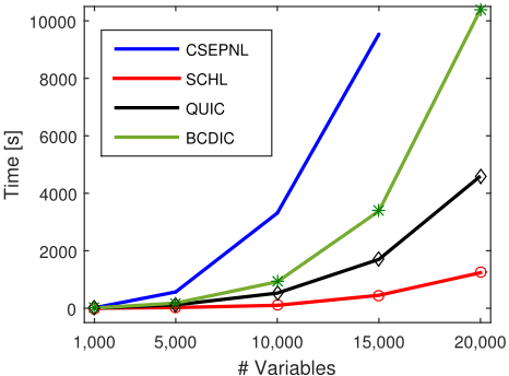
For our evaluation of computational efficiency, we replicated settings used in [Hsieh et al., 2011]. We constructed sparse adjacency matrices with randomly assigned off-diagonal nonzero entries. We ensured positive definiteness of the adjacency matrices by making them diagonally dominant. Subsequently, we used such matrices to generate a certain number of samples, from which the approaches should learn the inverse covariance matrix. Samples were randomly selected from multivariate Gaussian distribution and "colored" with a designed adjacency matrix to assure the underlying structure in observations. We generated several problems of varying sizes using the underlying structure of a random graph. Graph sizes spanning 1,000 to 20,000 nodes (variables) were selected in order to characterize the computational efficiency and scalability of competing approaches. In sparse random graph datasets the average node degree was set to belong in the interval of 15-20. In each experiment, an empirical covariance matrix was created from 1000 samples generated from a multivariate normal distribution with zero mean and a corresponding precision matrix. All experiments were conducted in a single thread Intel(R) Core(TM) i7-4770 CPU@ 3.40GHz machine with 32 GB RAM. Results can be seen at Figure 1, and additional details are provided in Table 1. Synthetic problems were generated to contain a certain amount of edges in the connectivity graph. In the evaluation of competing algorithms, we tuned the penalty parameter λ such that each approach learns the structure with a number of non-zero elements ("nnz") close to the targeted sparsity (true number of non-zeros). The results provide evidence that our SCHL algorithm is fastest, and scales better with the increase in a number of variables. According to the literature [Treister and Turek, 2014], BCDIC is expected to be faster than QUIC, however, in our study it is slower, most probably because our problem setups are denser.
Since we know the underlying process generating synthetic observations, we were able to characterize how well the algorithms uncovered the structure. We quantified the quality of obtained solutions by comparing the learned precision matrix with the ground truth. The measures used are Jaccard Index, precision, recall and accuracy to quantify the overlap of true and estimated nonzero elements, and R2 for assessing how well the magnitudes are replicated. For computational evaluation we generated one problem of size 10,000 with the underlying structure of a chain graph, from which we sampled 1,000 samples for precision matrix estimation. The results are provided in Table 2 and it can be seen that all approaches produced solutions of comparable quality. The sparsities of particular methods (nnz - est) were independently adjusted to approximately match the ground truth (nnz - true).
| SCHL | QUIC | BCDIC | CSEPNL | |
|---|---|---|---|---|
| time | 5,038.6 | 10,011.0 | 15,929.1 | 26,665.7 |
| nnz | 366,064 | 346,536 | 346,516 | 357,812 |
4.2 Structure Discovery Application
Advances in measuring technology allowed an abundance in the amount and especially in the dimensionality of data, increasing the need for automatic and unsupervised discovery of dependencies between the variables. This fosters application of learning approaches like SCHL on data from various domains, to uncover previously unknown connections and regularities. In the following text, we present application of our SCHL method to discover the connectivity structure on real world dataset from biomedical domain.
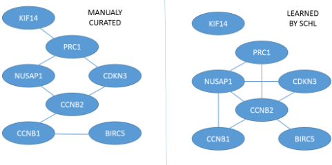
Gene Expression in Septic Patients The dataset contains whole blood gene expression profiles collected daily for up to 5 days from 53 subjects [Parnell et al., 2013]. A total of 163 samples was taken during the course of the experiment from patients that were admitted to the ICUs of hospitals in Sydney, Australia, with a diagnosis of sepsis. Measurements consist of expression levels of 24,840 probes (genes), and obtained gene expression levels were quantile normalized and log transformed. We have applied our SCHL approach on all 163 samples to discover the dependence structure between expression levels of human genes in sepsis, and again SCHL was fastest among the compared approaches (Table 3). In the conducted experiment we set the sparsity to an appropriately high level and obtained the co-expression network of 170,612 edges (out of possible 308,500,380). To check the plausibility of the obtained co-expression network, we looked at published literature for an example of a manually curated network of genes relevant to sepsis condition. We took the network of 7 genes connected by 7 links [Wang et al., 2016], that were obtained by literature mining and which were associated with a sepsis-related acute respiratory distress syndrome. In the network derived by our SCHL approach, subnetwork of these 7 genes contains 8 edges. The two networks are depicted at Figure 2, and it can be seen that 4 links are overlapping, which makes a solid recall. Given high sparsity of our co-expression network of just 0.05%, 7 node subgraph with 8 links makes 689-fold enrichment (only 0.0116 links expected), and is statistically highly unlike to happen by chance. These results provide evidence that SCHL can be used for constructing reliable co-expression networks, which are of high biological interest as co-expressed genes are functionally related, often involved in the same pathways [Stuart et al., 2003] or controlled by the same regulatory process important for therapeutic interventions [Stojkovic et al., 2016a].
5 Conclusions
We developed the SCHL, a novel approach for learning the sparse GMRFs. The SCHL model was built from a suitable reparametrization based on Cholesky decomposition. The new method is convex and can be efficiently optimized using coordinate descent with an active set approach. We show that SCHL is faster than the state-of-the-art approaches QUIC, BCDIC and CSEPNL on several examples and demonstrate its applicability in network discovery. As presented approach solves very general and widespread problem it can be further extended for supervised tasks like structured regression [Stojkovic et al., 2016b; Wytock and Kolter, 2013].
Acknowledgments
This research was supported in part by DARPA grant FA9550-12-1-0406 negotiated by AFOSR, DARPA and the ARO grant No. W911NF-16-C-0050, DARPA grant No. 66001-11-1-4183 negotiated by SSC Pacific grant, NSF BIGDATA grant 14476570 and ONR grant N00014-15-1-2729.
A Convexity
Theorem 1. The following function is convex:
where |L|= [ |Lij | ] is the matrix elementwise absolute value. Proof. While individual terms indeed are non-convex, the penalty term as a whole is convex, for positive semi-definite Λ matrix. First, we observe smooth regions of function h(L) where Lij ̸= 0, ∀(i, j). Since Λ matrix is PSD, it can be Cholesky decomposed: Λ = V V T , and using trace algebra, penalty (19) becomes:
which is a squared Frobenius norm of matrix V T |L| and, therefore, the function is convex inside each differentiable region (since the sign doesn't change).
Next, two neighboring smooth regions are separated with non-differentiable region defined when one of the parameters Lij is zero. It can be easily shown that the left derivative limLij→-0 ∂h(Lij ) ∂Lij is always smaller or equal to the right derivative limLij→+0 ∂h(Lij ) ∂Lij , granting the convexity to the penalty term as whole.
Here we use positive scalar lambda, which is PSD.
@inproceedings{ijcai2017p384,
  title     = {Fast Sparse Gaussian Markov Random Fields Learning Based on Cholesky Factorization},
  author    = {Stojkovic, Ivan and Jelisavcic, Vladisav and Milutinovic, Veljko and Obradovic, Zoran},
  booktitle = {Proceedings of the Twenty-Sixth International Joint Conference on
               Artificial Intelligence, {IJCAI-17}},
  publisher = {International Joint Conferences on Artificial Intelligence Organization},
  editor    = {Carles Sierra},
  pages     = {2758--2764},
  year      = {2017},
  month     = {8},
  note      = {Main track},
  doi       = {10.24963/ijcai.2017/384},
  url       = {https://doi.org/10.24963/ijcai.2017/384},
}
TY - CPAPER TI - Fast Sparse Gaussian Markov Random Fields Learning Based on Cholesky Factorization AU - Stojkovic, Ivan AU - Jelisavcic, Vladisav AU - Milutinovic, Veljko AU - Obradovic, Zoran T2 - Proceedings of the Twenty-Sixth International Joint Conference on Artificial Intelligence, IJCAI-17 PB - International Joint Conferences on Artificial Intelligence Organization PY - 2017 SP - 2758 EP - 2764 DO - 10.24963/ijcai.2017/384 UR - https://doi.org/10.24963/ijcai.2017/384 ER -Copied
Machine-readable versions of this paper, for tools and AI agents:





