
Adaptive Semi-Supervised Learning with Discriminative Least Squares Regression
Proceedings of the Twenty-Sixth International Joint Conference on Artificial Intelligence. Main track. Pages 2421-2427.
https://doi.org/10.24963/ijcai.2017/337
Keywords
- Machine Learning: Semi-Supervised Learning
- Machine Learning: Machine Learning
Abstract
Semi-supervised learning plays a significant role in multi-class classification, where a small number of labeled data are more deterministic while substantial unlabeled data might cause large uncertainties and potential threats.
In this paper, we distinguish the label fitting of labeled and unlabeled training data through a probabilistic vector with an adaptive parameter, which always ensures the significant importance of labeled data and characterizes the contribution of unlabeled instance according to its uncertainty. Instead of using traditional least squares regression (LSR) for classification, we develop a new discriminative LSR by equipping each label with an adjustment vector. This strategy avoids incorrect penalization on samples that are far away from the boundary and simultaneously facilitates multi-class classification by enlarging the geometrical distance of instances belonging to different classes. An efficient alternative algorithm is exploited to solve the proposed model with closed form solution for each updating rule. We also analyze the convergence and complexity of the proposed algorithm theoretically. Experimental results on several benchmark datasets demonstrate the effectiveness and superiority of the proposed model for multi-class classification tasks.
- [Belkin et al., 2006] Mikhail Belkin, Partha Niyogi, and Vikas Sindhwani. Manifold regularization: A geometric framework for learning from labeled and unlabeled exam- ples. J. Mach. Learn. Res., 7:2399-2434, 2006.
- [Bishop, 2006] Christopher M Bishop. Pattern recognition. Mach. Learn., 128:1-58, 2006.
- [Cai et al., 2007a] Deng Cai, Xiaofei He, and Jiawei Han. Semi-supervised discriminant analysis. In ICCV, 2007.
- [Cai et al., 2007b] Deng Cai, Xiaofei He, Yuxiao Hu, Jiawei Han, and Thomas Huang. Learning a spatially smooth sub- space for face recognition. In CVPR, 2007.
- [Chang and Yang, 2016] Xiaojun Chang and Yi Yang. Semisupervised feature analysis by mining correlations among multiple tasks. IEEE Trans. Neural Netw. Learn. Syst., 2016.
- [Chang et al., 2014] Xiaojun Chang, Feiping Nie, Yi Yang, and Heng Huang. A convex formulation for semi- supervised multi-label feature selection. In AAAI, 2014.
- [Chapelle et al., 2008] Olivier Chapelle, Vikas Sindhwani, and Sathiya S Keerthi. Optimization techniques for semi- supervised support vector machines. J. Mach. Learn. Res., 9:203-233, 2008.
- [Chapelle et al., 2009] Olivier Chapelle, Bernhard Scholkopf, and Alexander Zien. Semi-supervised learning. IEEE Trans. Neural Netw., 20(3):542-542, 2009.
- [Fan et al., 2005] Rong-En Fan, Pai-Hsuen Chen, and Chih- Jen Lin. Working set selection using second order infor- mation for training support vector machines. J. Mach. Learn. Res., 6:1889-1918, 2005.
- [Georghiades et al., 2001] Athinodoros S Georghiades, Pe- ter N Belhumeur, and David J Kriegman. From few to many: Illumination cone models for face recognition un- der variable lighting and pose. IEEE Trans. Pattern Anal. Mach. Intell., 23(6):643-660, 2001.
- [Liu et al., 2011] Xiaobai Liu, Xiaotong Yuan, Shuicheng Yan, and Hai Jin. Multi-class semi-supervised svms with positiveness exclusive regularization. In ICCV, 2011.
- [Luo et al., 2017] Minnan Luo, Xiaojun Chang, Liqiang Nie, Yi Yang, Alexander G Hauptmann, and Qinghua Zheng. An adaptive semisupervised feature analysis for video se- mantic recognition. IEEE Trans. Cybern., 2017.
- [Nie et al., 2010] Feiping Nie, Dong Xu, Ivor Wai-Hung Tsang, and Changshui Zhang. Flexible manifold em- bedding: A framework for semi-supervised and unsuper- vised dimension reduction. IEEE Trans. Image Process., 19(7):1921-1932, 2010.
- [Nie et al., 2011a] Feiping Nie, Hua Wang, Heng Huang, and Chris Ding. Unsupervised and semi-supervised learn- ing via ℓ 1 -norm graph. In ICCV, 2011.
- [Nie et al., 2011b] Feiping Nie, Dong Xu, Xuelong Li, and Shiming Xiang. Semisupervised dimensionality reduction and classification through virtual label regression. IEEE Trans. Systems, Man, and Cybernetics, Part B, 41(3):675- 685, 2011.
- [Sim et al., 2002] Terence Sim, Simon Baker, and Maan Bsat. The cmu pose, illumination, and expression (pie) database. In FG, 2002.
- [Sindhwani and Keerthi, 2006] Vikas Sindhwani and S Sathiya Keerthi. Large scale semi-supervised linear svms. In ACM SIGIR, 2006.
- [Subramanya and Talukdar, 2014] Amarnag Subramanya and Partha Pratim Talukdar. Graph-based semi-supervised learning. Synthesis Lectures on Artificial Intelligence and Machine Learning, 8(4):1-125, 2014.
- [Wang et al., 2014] De Wang, Feiping Nie, and Heng Huang. Large-scale adaptive semi-supervised learning via unified inductive and transductive model. In SIGKDD, 2014.
- [Xiang et al., 2012] Shiming Xiang, Feiping Nie, Gaofeng Meng, Chunhong Pan, and Changshui Zhang. Discrimi- native least squares regression for multiclass classification and feature selection. IEEE Trans. Neural Netw. Learn. Syst., 23(11):1738-1754, 2012.
- [Yan et al., 2007] Shuicheng Yan, Dong Xu, Benyu Zhang, Hong-Jiang Zhang, Qiang Yang, and Stephen Lin. Graph embedding and extensions: a general framework for di- mensionality reduction. IEEE Trans. Pattern Anal. Mach. Intell., 29(1):40-51, 2007.
- [Yang et al., 2015] Yi Yang, Zhigang Ma, Feiping Nie, Xiao- jun Chang, and Alexander G Hauptmann. Multi-class ac- tive learning by uncertainty sampling with diversity maxi- mization. Int. J. Comput. Vision, 113(2):113-127, 2015.
- [Zhou et al., 2004] Dengyong Zhou, Olivier Bousquet, Thomas Navin Lal, Jason Weston, and Bernhard Schölkopf. Learning with local and global consistency. NIPS, 2004.
- [Zhu and Goldberg, 2009] Xiaojin Zhu and Andrew B Gold- berg. Introduction to semi-supervised learning. Morgan & Claypool Publishers, 2009.
- [Zhu et al., 2003] Xiaojin Zhu, Zoubin Ghahramani, John Lafferty, et al. Semi-supervised learning using gaussian fields and harmonic functions. In ICML, 2003.
- [Zhu et al., 2004] Xiaojin Zhu, Jaz Kandola, Zoubin Ghahramani, and John D Lafferty. Nonparametric trans- forms of graph kernels for semi-supervised learning. In NIPS, 2004.
References were extracted automatically from the PDF and may contain errors.
Full text extracted automatically from the PDF; figures, tables and equations may differ. The PDF is the version of record.
1 Introduction
Data are abundant due to the digital information explosion. However, a vast majority of large-scale data are usually collected without labels for classification. Labeling these data requires the efforts of human annotators who must often be quite skilled [Zhu et al., 2003; Yang et al., 2015]. Moreover, this process is difficult to scale and often error prone for its dramatically expensive and time-consuming cost [Subramanya and Talukdar, 2014; Chang et al., 2014; Luo et al., 2017]. As a result, it is crucial to develop semisupervised learning (SSL) algorithms which potentially improve the generalization performance by employing a small amount of labeled data jointly with a large number of unlabeled data [Chapelle et al., 2008; Zhu and Goldberg, 2009; Chang and Yang, 2016].
∗Corresponding author: Feiping Nie (feipingnie@gmail.com)
In the past decades, researchers have proposed a variety of semi-supervised learning algorithms. Most of them are started by representing the training data (labeled and unlabeled) as a graph and assume that data points are likely to have the same label if they are close to each other [Chapelle et al., 2009]. For example, semi-supervised support vector machines (SVMs) with manifold regularization [Sindhwani and Keerthi, 2006; Belkin et al., 2006; Liu et al., 2011], graph kernels based SSL [Zhu et al., 2004], semi-supervised discriminant analysis from graph perspective [Cai et al., 2007a], SSL with local and global consistency [Zhou et al., 2004], gaussian eld harmonic function [Zhu et al., 2003] and so on. Since data points from different classes can be quite close in practice, the graph-based algorithms might fail to achieve desirable performance when two classes overlap significantly [Zhu and Goldberg, 2009]. Additionally, conventional semisupervised learning algorithms treat the labeled and unlabeled instances equally in the training stage. In fact, the labeled data are usually more deterministic and should play a more significant role, while substantial unlabeled data might cause large uncertainties and potential threats. Thus, it is crucial to distinguish between different label types of training instances in the framework of SSL [Nie et al., 2011b]. Wang et al. [Wang et al., 2014] introduced an adaptive parameter to suppress the weights of unlabeled data points around the boundary. However, this method employs traditional least squares regression (LSR) loss function for classification, which usually penalizes the data points far away from the boundary even when they are classified correctly for sure [Bishop, 2006; Xiang et al., 2012].
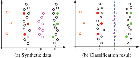
In this paper, we exploit an adaptive semi-supervised classification algorithm with a novel discriminative LSR. This idea is illustrated by a synthetic dataset (see Figure 1a) consisting of labeled data points (filled circles from two classes) and unlabeled ones (hollow circles). Specifically, the unlabeled data points with various uncertainties include the purple ones around the boundary, the brown ones far away from the boundary, and the black ones following the distribution of the labeled data. By assigning a probabilistic vector to the fitting of each sample, our method always ensure the significant importance of labeled data while characterizing the contribution of the unlabeled instance according to its uncertainty. See the classification performance of our model in Figure 1b. The size of labeled data remain unchanged, while the unlabeled data points with comparable deterministic affiliation become smaller. Specifically the unlabeled data points around the boundary that belong to multiple labels with similar probabilities turn to be much smaller. To overcome the shortcomings of the conventional LSR for classification, we equip each label with an adjustment vector. This strategy prevents the incorrect penalization of unlabeled samples far away from the boundary. As a result, our model performs robust to not only the unlabeled data with varying uncertainties but also the outliers far away from the boundary. In summary, we describe the contributions of this paper as follows:
- We associate each label with an adjustment vector and develop a new discriminative LSR to prevent incorrect penalization on the data far away from the boundary.
- Based on the proposed discriminative LSR, we concern the contribution difference of training data in semisupervised learning and developed a unified label fitting for both labeled and unlabeled training data.
- We exploit an efficient alternative algorithm to solve the proposed model with closed form solution for each updating rule, and analyze its convergence and computational complexity theoretically.
2 The ProposedMethodology
In this section, we first introduce a new discriminative least squares regression, and then propose an adaptive framework for semi-supervised classification.
2.1 Discriminative LSR
In this paper, we denote the training set by X = {x1, x2, · · · , xn}, where xi ∈ Rd is the feature vector of the i-th instance. In the framework of semisupervised classification, we suppose the first nl(nl ≤ n) instances, i.e., x1, x2, · · · , xnl , are labeled uniquely c different classes. The remaining nu = n - nl instances, i.e., xnl+1, xnl+2, · · · , xn, are unlabeled. To identify the c classes uniquely, we associate the k-th class with a coding tk = [-1, · · · ,-1, 1,-1, · · · ,-1]⊤ ∈ Rc , where only the k-th element of tk is equal to 1 and the other ones are -1.
Instead of using traditional regression loss which usually incorrectly penalizes the right classification, in this paper, we take tk (k = 1, 2, · · · , c) as the regression target and associate each class with an adjustment variable mk = [mk1,mk2, · · · ,mkc]⊤ ≥ 0 (k = 1, 2, · · · , c). Let W ∈ Rd×c be a transformation matrix and b ∈ Rc be a bias vector, the proposed discriminative regression loss (fitting loss) for the i-th instance which belongs to the k-th class is defined as
where ⊙ is a Hadamard product operator of vectors. In contrast to the traditional regression loss, the introduced term tk ⊙mk are capable of not only offsetting the incorrect penalization but also enlarging the margin between classes. For a better representation, we collect all of adjustment variables into matrix M = [m1,m2, · · · ,mc] ∈ Rc×c . We take the instance xi ∈ R3 which might belong to one of c = 3 different classes for example. The discriminative regression loss of xi belonging to the 2-th class is formulated as
where zi = [zi1, zi2, zi3]⊤ is the predicted label vector for xi. If xi belongs to the 2-th class with the predicted label vector zi ≫ t2, the value of loss Di2 keeps small with an appropriate non-negative adjustment variable m2. This strategy effectively prevents the correct classification from being penalized. Moreover, the introduced nonnegative variablem2 intuitively enlarge the distance between different classes in the projected space as much as possible. Note that the proposed discriminative LSR is more efficient and usually have better generalization ability than the one in [Xiang et al., 2012] which associates each instance with c non-negative variables.
2.2 Semi-supervised Classification with DLSR
Taking the advantages of discriminative LSR, we consider the contribution importance of varying training data in the framework of semi-supervised learning and propose a novel fitting loss for both labeled and unlabeled data in a unified formulation, i.e.,
where yik ∈ [0, 1]c (i = 1, 2 · · · , n; k = 1, 2, · · · , c) refers to the probability of the i-th instance belonging to the k-th class. For a training instance xi ∈ X with probability vector yi = [yi1, yi2, · · · , yic] ∈ [0, 1]c , its contribution importance is defined as
where r ≥ 1 is an adaptive parameter. The advantages of this definition are embodied in the following three aspects. Firstly, it ensures the significance of labeled data since the contribution importance of any labeled instance is always 1 for any adaptive parameter r ≥ 1. Secondly, it is capable of reflecting how much proportions of the unlabeled data play at the macro level because, on one hand, the unlabeled instance is considered to have the equal importance as labeled data when the adaptive parameter r → 1; On the other hand, the unlabeled instance has no effect on the training stage as the adaptive parameter r →∞. Thirdly, the contribution importance with fixed 1 < r < ∞ can distinguish between different types of unlabeled data at the micro level. This setting coincides with the fact that uncertain unlabeled instances should have less influence on the procedure of training. In summary, the contribution importance not only distinguish between labeled and unlabeled instances at the macro level but also differentiate the varieties of unlabeled data at the micro level.
Let Y = [Yl; Yu] ∈ [0, 1]n×c be the probability matrix for training data, where Yl = [y1, y2, · · · , ynl ]⊤ ∈ [0, 1]nl×c and Yu = [ynl+1, ynl+2, · · · , yn]⊤ ∈ [0, 1]nu×c refer to the probability matrices of labeled and unlabeled data, respectively. We employ the loss function (1) and formulate the idea of semi-supervised classification with discriminative LSR as the following optimization problem
where Ω = {W, b, Yu,M} collects all of the optimization variables. r ≥ 1 is the adaptive parameter which needs to be tuned; The regularization ‖W‖2F controls the complexity of model with a trade-off parameter λ. In contrast to the approach used in [Wang et al., 2014], the proposed optimization problem (2) not only demonstrates excellent robustness to the unlabeled uncertainty instances that are near the classification boundary but also prevents the correct classification from being penalized.
3 Optimization Procedure
In this section, we exploit a simple and efficient alternative algorithm to solve the proposed optimization problem (2), and analyze its computational complexity and convergence theoretically.
3.1 Optimize Unlabeled ProbabilityMatrix Yu:
Consider the independence of training data, probability vector for each instance can be updated simultaneously by solving the following optimization problem
where Dik = Dik(W, b, mk; xi) is calculated with fixed parameters W, b and mk (k = 1, 2, · · · , c). If the adaptive parameter r is set to 1, the optimization problem (3) has a trivial solution
for k = 1, 2, · · · , c. In this case, the labeled data and unlabeled data are treated equally in the semi-supervised classification. For a more general case that r > 1, let the Lagrangian function of objective (3) be Lα = ∑ck=1 yr ikDik - α(∑ck=1 yik - 1), where α is the Lagrangian multiplier. Setting the derivative of Lagrangian function Lα in terms of yik to zero and combining with the constraint ∑ck=1 yik = 1, we arrive at the following closed-form solution for optimization problem (3)
Given this closed-form solution, the optimal probability vector for each unlabeled instance is updated efficiently.
3.2 Optimize W and b:
To update W and b with fixed Y and M, we frist introduce the following Theorem 1.
Theorem 1. Given W ∈ Rd×c , b ∈ Rc , Y ∈ Rn×c and M ∈ Rc×c , let T = [t1, t2, · · · , tc] ∈ Rc×c and H = T +T ⊙M. The loss function L(W, b,M, Y ) can be reformulated as a compact matrix representation
where Ω = diag(ωr 1 , ωr 2 , · · · , ωrn ) ∈ Rn×n is a diagonal matrix with its (i, i)-th diagonal element being the contribution importance of the i-th instance; F = Y r is computed in element wise; G = diag(g11, g22, · · · , gcc) ∈ Rc×c is also a diagonal matrices with its (k, k)-th diagonal element being gkk = ∑ni=1 yr ik (k = 1, 2, · · · , c).
Proof. The result is derived with some matrix theories.
Based on Theorem 1, we update W and b according to the following Theorem 2.
Theorem 2. Given fixed parameters Y andM, the solutions of optimization problem (2) with respect to variables W and b are derived as the following closed forms
where P = In - 1n1⊤n Ω/1⊤n Ω1n ∈ Rn×n ; Id and In are identity matrices of size d × d and n × n, respectively.
Proof. According to Theorem 1, the optimal W and b can be achieved through minimizing the objective function f (W, b) = T r [(W ⊤X + b1⊤n )Ω(W ⊤X + b1⊤n )⊤] -
2T r [FH⊤(W ⊤X + b1⊤n )]+λ‖W‖2F . By some matrix theories, we set the derivative of f (W, b) with respect to variable b to zero, i.e.,
Thus, we have b = (HF ⊤ -W ⊤XΩ)1n/1⊤n Ω1n. Moreover, setting the derivative of f(W, b) with respect to variable W to zero, i.e.,
and substituting the derivation of b into the equation above, we arrive at
where P = In - 1n1⊤n Ω/1⊤n Ω1n. As a result, the optimal W is obtained in a closed form W = (XΩPX⊤ + λId)-1XP ⊤FH⊤. The proof is completed.
3.3 Optimize Adjustment Variable M:
Given W, b and Y , the optimal M can be obtained through solving problem minM≥0 L(W, b,M, Y ). To this end, we introduce the following Theorem 3.
Theorem 3. Given W ∈ Rd×c , b ∈ Rc and Y ∈ Rn×c , let F = Y r ∈ Rn×c be calculated in element wise; G = diag(g11, g22, · · · , gcc) ∈ Rc×c be a diagonal matrix with its (k, k)-th element gkk = ∑ni=1 yr ik (k = 1, 2, · · · , c). The solution of optimization problem (2) with respect to M is derived as a closed form
Proof. According to the compact matrix representation of loss function L(W, b,M, Y ) in Theorem 1, we denote H = T + T ⊙M with T = [t1, t2, · · · , tc] ∈ Rc×c , and compute the derivative of L(W, b,M, Y ) with respect to M, i.e.,
Recall that matrix T is invertible, we set the derivative of L(W, b,M, Y ) to 0, and thus obtain
Since the (k, k)-th element of T is 1 and the others are -1 for k = 1, 2, · · · , c, T ⊙ T = 1c×c holds, where 1c×c refers to a matrix whose elements are all 1. Thus we have M = T ⊙ [(W ⊤X + b1⊤n )FG-1 - T ]. The proof is completed.
In summary, we describe the alternative algorithm for optimization problem (2) in Algorithm 1. Because of the closedform solutions to each updating rule, Algorithm 1 is very simple to implement and efficient to run on large scale datasets. Specifically, the overall computational cost of Algorithm 1 is less than O(Td2 c) + O(nd2 ) + O(ndc). For real world application, since the number of classes c is always much smaller than the dimensionality of data d and the number of data points n, the upper bound computational cost reduces to O(Td2 ) +O(nd2 ). We also analyze the convergence of the proposed algorithm in the following Theorem 4.
Algorithm 1 Alternative optimization for problem (2)
Input: X = [Xl;Xu] ∈ Rd×n with label matrix Fl ∈ Rnl×c ; λ; r ≥ 1.
Initialization: W (0) ∈ Rd×c , b(0) ∈ Rc , M (0) ∈ Rc×c and
t = 0.
- 1: while not converge do
- 2: Update Y t+1 u given W (t) , b(t) and M (t) by Eq. (4) if r = 1, by Eq. (5) otherwise;
- 3: Update W (t+1) and bt+1 given Y t+1 and M t by Eq. (6) and Eq. (7);
- 4: Update M (t+1) given W (t+1) , b(t+1) and Y (t+1) by Eq. (9);
- 5: t = t + 1;
- 6: end while
Theorem 4. The iterative updating rules in Algorithm 1 monotonically decrease the objective function value of the optimization problem (2) in each iteration until convergence.
Proof. Let the value of objective function (2) be F(W (t) , b(t) ,M (t) , Y (t) ) = L(W (t) , b(t) ,M (t) , Y (t) )+ λ‖W (t) ‖2F at the t-th iteration. In alternative optimization Algorithm 1, since we update variable Y with closed-form solution by Y (t+1) = argminY L(W (t) , b(t) ,M (t) , Y ), followed by updating variables W and b according to (W (t+1) , b(t+1) ) = argminW,b F(W, b,M (t) , Y (t+1) ), the inequality F(W (t+1) , b(t+1) ,M (t) , Y (t+1) ) ≤ F(W (t) , b(t) ,M (t) , Y (t) ) holds evidently. Furthermore, the adjustment variable M is updated through M (t+1) = argminM L(W (t+1) , b(t+1) ,M, Y (t+1) ), we have F(W (t+1) , b(t+1) ,M (t+1) , Y (t+1) ) ≤ F(W (t) , b(t) ,M (t) , Y (t) ). Recall objective function (2) is bounded below, thus its value decrease monotonically in each iteration until Algorithm 1 convergence.
4 Experiment
In this section, several benchmark datasets of varying image types are used to validate the effectiveness and superiority of the proposed model, including the ORL database of faces [Cai et al., 2007b], the extended Yale B database (YaleB) of face [Georghiades et al., 2001], the face database CMU-PIE [Sim et al., 2002] and the palm print database (PALM) [Yan et al., 2007]. We download all of the datasets from different websites. The pixel value of the image is used as its feature representation. Images of the faces are resized to 32 × 32 while the palm print images in PALM are resized to 16 × 16.
We compare the proposed model with some state-of-the-art classification methods, including supervised learning methods: SVM [Fan et al., 2005] and classification based on discriminative LSR (SDLSR) with respect to each data points [Xiang et al., 2012], transductive learning methods: Semisupervised classification with Gaussian Fields and Harmonic Functions (GFHF) [Zhu et al., 2003] and Semi-Supervised Learning with ℓ1-Norm Graph (ℓ1-SEMI) [Nie et al., 2011a], two inductive learning: semi-supervised learning with Flexible Manifold Embedding (FME) [Nie et al., 2010] and Adaptive Semi-Supervised Learning (ASL) [Wang et al., 2014].
| ORL | YaleB | CMU-PIE | PALM | |||||
|---|---|---|---|---|---|---|---|---|
| Unlabeled | Testing | Unlabeled | Testing | Unlabeled | Testing | Unlabeled | Testing | |
| SVM | 0.513±0.027 | 0.501±0.014 | 0.187±0.015 | 0.187±0.021 | 0.276±0.012 | 0.279±0.015 | 0.801±0.012 | 0.811±0.013 |
| SDLSR | 0.660±0.028 | 0.658±0.023 | 0.937±0.007 | 0.940±0.010 | 0.895±0.013 | 0.900±0.012 | 0.925±0.008 | 0.931±0.012 |
| GFHF | 0.614±0.023 | NA | 0.582±0.022 | NA | 0.654±0.008 | NA | 0.914±0.012 | NA |
| ℓ1-SEMI | 0.576±0.016 | NA | 0.387±0.026 | NA | 0.553±0.031 | NA | 0.891±0.013 | NA |
| FME | 0.665±0.018 | 0.672±0.014 | 0.928±0.008 | 0.933±0.012 | 0.881±0.015 | 0.884±0.015 | 0.942±0.008 | 0.945±0.012 |
| ASL | 0.674±0.020 | 0.666±0.013 | 0.964±0.004 | 0.962±0.004 | 0.943±0.009 | 0.946±0.008 | 0.963±0.010 | 0.964±0.015 |
| Our Model | 0.718±0.012 | 0.725±0.012 | 0.996±0.001 | 0.995±0.002 | 0.954±0.005 | 0.957±0.006 | 0.982±0.005 | 0.986±0.007 |
| ORL | YaleB | CMU-PIE | PALM | |||||
|---|---|---|---|---|---|---|---|---|
| Unlabeled | Testing | Unlabeled | Testing | Unlabeled | Testing | Unlabeled | Testing | |
| SVM | 0.521±0.014 | 0.514±0.026 | 0.315±0.030 | 0.319±0.033 | 0.378±0.012 | 0.383±0.011 | 0.917±0.007 | 0.921±0.009 |
| SDLSR | 0.662±0.018 | 0.662±0.017 | 0.982±0.002 | 0.981±0.003 | 0.955±0.013 | 0.957±0.009 | 0.986±0.005 | 0.988±0.003 |
| GFHF | 0.627±0.023 | NA | 0.735±0.020 | NA | 0.800±0.008 | NA | 0.981±0.004 | NA |
| ℓ1-SEMI | 0.584±0.024 | NA | 0.576±0.016 | NA | 0.768±0.031 | NA | 0.976±0.005 | NA |
| FME | 0.672±0.018 | 0.689±0.023 | 0.990±0.003 | 0.989±0.003 | 0.952±0.015 | 0.953±0.008 | 0.989±0.004 | 0.991±0.003 |
| ASL | 0.691±0.027 | 0.689±0.013 | 0.996±0.002 | 0.995±0.002 | 0.969±0.009 | 0.968±0.004 | 0.992±0.005 | 0.993±0.005 |
| Our Model | 0.732±0.012 | 0.736±0.021 | 0.997±0.001 | 0.997±0.002 | 0.973±0.005 | 0.974±0.005 | 0.994±0.005 | 0.996±0.004 |
For each dataset, two thirds of samples are randomly selected as the training data, while the remaining ones are served as the testing data. At the semi-supervised training stage, we randomly choose only 10% or 20% samples with labels. For the regularization parameter used in SDLSR, ℓ1SEMI, FME , ASL and our model, we tune them in the range of {10-3 , 10-2 , 10-1 , 100 , 101 , 102 , 103 } and report the best results. Following [Nie et al., 2010], we use the Gaussian function to compute the Laplacian matrix for all graph-based methods. The adaptive parameter used in ASL and our model is tuned from 1 to 2 with a step-size of 0.1.
4.1 Experimental Results Comparison
For a fair comparison, we randomly split each dataset into training and testing dataset 50 times and report the average accuracy with standard deviation (STD) for the unlabeled data in training dataset and testing data. The experimental results on four datasets are collected in Table 1 and Table 2 with 10% and 20% labeled samples, where "NA" indicates that transductive semi-supervised classification approaches are not able to predict labels for samples out of training stage. From the experimental comparison, we have the following observations. (1) The performance of each algorithm becomes better as the increase of labeled data in the training stage. This phenomenon looks more obvious in supervised and transductive semi-supervised classification than inductive semi-supervised learning algorithms. (2) Thanks to the information proved by unlabeled data, the performance of semi-supervised classification algorithms exceeded SVM. However, both running in the supervised scenario, SDLSR achieves much better results than SVM. In fact, the performance of SDLSR is even over transductive semi-supervised classification approaches since it concerns the discriminative variables of each label for each samples. (3) Since our model takes the contribution importances of different training data into consideration, together with the introduced adjustment variables for each label, it consistently outperforms other methods over all datasets. ASL also considers the contribution importances but achieves the second best performance because it employs traditional LSR for classification.
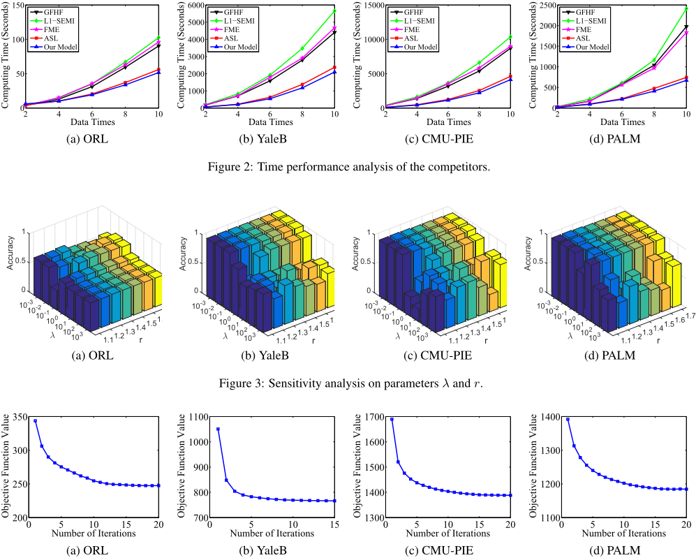
We also conduct some numeric experiments to verity the time superiority of the proposed algorithm. With 20% labeled training data, we copy each datasets 2-times, 4-times, 6-times, 8-times and 10-times respectively and report the time performance over each extended datasets in Figure 2. Note that because ℓ1-SEMI, ASL and our model are solved through alternative optimization algorithm, a equal convergence residual is shared for a fair comparison. We observe from the experimental result that: (1) The time cost of the graph-based methods, including GFHF, ℓ1-SEMI and FME grow more rapidly than the proposed model and ASL with the increase of training data; (2) Our model consumes less time than other semi-supervised methods, especially when the number of data increases larger. This result gears to the computational complexity mentioned above and demonstrates the efficiency of the proposed model for large scale data applications.
4.2 Sensitivity and Convergence
To illustrate the influence of parameters on the performance of semi-supervised classification, we report in Figure 3 the performance of the proposed model with varying values of parameters λ ∈ [10-3 , 103 ] with step-size of 10 and r ∈ [1.1, 1.7] with step-size of 0.1. We observe from the experimental results that the performance varies with different settings on various datasets. As a result, how to identify the optimal values of the parameters is data dependent. Generally, the results could be satisfactory and relatively stable when λ and r fall in the range of [10-2 , 10-1 ] and [1.5, 1.7], respectively. To illustrate the efficiency of our algorithm, we plot the corresponding convergence curves of the objective function (2) for two datasets in Figure 4, where the parameters λ and r are set as 0.1 and 1.4, respectively; 20% labeled data are involved in the training stage. It is evident that our algorithm converges within 20 iterations over all datasets, validating the efficiency and quickly converges of this algorithm.
5 Conclusion
In this paper, we develop a new discriminative LSR where each label is associated with an adjustment variable to eliminate the penalty of data that are classified correctly. Based on this discriminative LSR, we propose a novel semi-supervised classification which concerns the contribution importance of labeled and unlabeled training data simultaneously. An efficient alternative algorithm is exploited to solve the proposed challenging problems with theoretical analyses on its convergence and computational complexity. Experimental results, including the performance of accuracy and time cost, demonstrate the superiority and efficiency of the proposed model.
Acknowledgments
This work was funded by the National Science Foundation of China (No.61502377), the National Key Research and Development Program of China (No.2016YFB1000903), China Postdoctoral Science Foundation (No. 2015M582662), Ministry of Education Innovation Research Team (No.IRT13035) Project of China Knowledge Centre for Engineering Science and Technology and the Project of No.41418070102.
@inproceedings{ijcai2017p337,
  title     = {Adaptive Semi-Supervised Learning with Discriminative Least Squares Regression},
  author    = {Luo, Minnan and Zhang, Lingling and Nie, Feiping and Chang, Xiaojun and Qian, Buyue and Zheng, Qinghua},
  booktitle = {Proceedings of the Twenty-Sixth International Joint Conference on
               Artificial Intelligence, {IJCAI-17}},
  publisher = {International Joint Conferences on Artificial Intelligence Organization},
  editor    = {Carles Sierra},
  pages     = {2421--2427},
  year      = {2017},
  month     = {8},
  note      = {Main track},
  doi       = {10.24963/ijcai.2017/337},
  url       = {https://doi.org/10.24963/ijcai.2017/337},
}
TY - CPAPER TI - Adaptive Semi-Supervised Learning with Discriminative Least Squares Regression AU - Luo, Minnan AU - Zhang, Lingling AU - Nie, Feiping AU - Chang, Xiaojun AU - Qian, Buyue AU - Zheng, Qinghua T2 - Proceedings of the Twenty-Sixth International Joint Conference on Artificial Intelligence, IJCAI-17 PB - International Joint Conferences on Artificial Intelligence Organization PY - 2017 SP - 2421 EP - 2427 DO - 10.24963/ijcai.2017/337 UR - https://doi.org/10.24963/ijcai.2017/337 ER -Copied
Machine-readable versions of this paper, for tools and AI agents:





