
Efficient Kernel Selection via Spectral Analysis
Proceedings of the Twenty-Sixth International Joint Conference on Artificial Intelligence. Main track. Pages 2124-2130.
https://doi.org/10.24963/ijcai.2017/295
Keywords
- Machine Learning: Classification
- Machine Learning: Data Mining
- Machine Learning: Kernel Methods
Abstract
Kernel selection is a fundamental problem of kernel methods. Existing measures for kernel selection either provide less theoretical guarantee or have high computational complexity. In this paper, we propose a novel kernel selection criterion based on a newly defined spectral measure of a kernel matrix, with sound theoretical foundation and high computational efficiency. We first show that the spectral measure can be used to derive generalization bounds for some kernel-based algorithms. By minimizing the derived generalization bounds, we propose the kernel selection criterion with spectral measure. Moreover, we demonstrate that the popular minimum graph cut and maximum mean discrepancy are two special cases of the proposed criterion. Experimental results on lots of data sets show that our proposed criterion can not only give the comparable results as the state-of-the-art criterion, but also significantly improve the efficiency.
- [Bartlett and Mendelson, 2002] Peter L. Bartlett and Shahar Mendelson. Rademacher and Gaussian complexities: risk bounds and structural results. Journal of Machine Learn- ing Research, 3:463-482, 2002.
- [Bartlett et al., 2005] Peter L. Bartlett, Olivier Bousquet, and Shahar Mendelson. Local Rademacher complexities. The Annals of Statistics, 33(4):1497-1537, 2005.
- [Bousquet and Elisseeff, 2002] Olivier Bousquet and André Elisseeff. Stability and generalization. Journal of Machine Learning Research, 2:499-526, 2002.
- [Cawley, 2006] Gavin C. Cawley. Leave-one-out cross- validation based model selection criteria for weighted LS- SVMs. In Proceeding of the International Joint Con- ference on Neural Networks (IJCNN 2006), pages 1661- 1668, 2006.
- [Chapelle et al., 2002] Olivier Chapelle, Vladimir Vapnik, Olivier Bousquet, and Sayan Mukherjee. Choosing mul- tiple parameters for support vector machines. Machine Learning, 46(1-3):131-159, 2002.
- [Cortes et al., 2010] Corinna Cortes, Mehryar Mohri, and Afshin Rostamizadeh. Two-stage learning kernel algo- rithms. In Proceedings of the 27th Conference on Machine Learning (ICML 2010), pages 239-246, 2010.
- [Cortes et al., 2013] Corinna Cortes, Marius Kloft, and Mehryar Mohri. Learning kernels using local Rademacher complexity. In Advances in Neural Information Process- ing Systems 25 (NIPS 2013), pages 2760-2768. MIT Press, 2013.
- [Cristianini et al., 2001] Nello Cristianini, John Shawe- Taylor, André Elisseeff, and Jaz S. Kandola. On kernel- target alignment. In Advances in Neural Information Pro- cessing Systems 14 (NIPS 2001), pages 367-373, 2001.
- [Debruyne et al., 2008] Michiel Debruyne, Mia Hubert, and Johan A.K. Suykens. Model selection in kernel based re- gression using the influence function. Journal of Machine Learning Research, 9:2377-2400, 2008.
- [Gao and Zhou, 2013] Wei Gao and Zhi-Hua Zhou. On the doubt about margin explanation of boosting. Artificial In- telligence, 203:1-18, 2013.
- [Golub et al., 1979] Gene H. Golub, Michael Heath, and Grace Wahba. Generalized cross-validation as a method for choosing a good ridge parameter. Technometrics, 21(2):215-223, 1979.
- [Gretton et al., 2007] Arthur Gretton, Karsten M. Borg- wardt, Malte Rasch, Bernhard Schölkopf, and Alexander J. Smola. A kernel method for the twosample problem. In Advances in Neural Information Processing Systems 15 (NIPS 2007), pages 513-520, 2007.
- [Kloft and Blanchard, 2011] Marius Kloft and Gilles Blan- chard. The local Rademacher complexity of lp-norm mul- tiple kernel learning. In Advances in Neural Information Processing Systems 23 (NIPS 2011), pages 2438-2446.
- [Kloft et al., 2011] Marius Kloft, Ulf Brefeld, Sören Son- nenburg, and Alexander Zien. Lp-norm multiple kernel learning. Journal of Machine Learning Research, 12:953- 997, 2011.
- [Lanckriet et al., 2004] Gert R. G. Lanckriet, Nello Cristian- ini, Peter L. Bartlett, Laurent El Ghaoui, and Michael I. Jordan. Learning the kernel matrix with semidefinite pro- gramming. Journal of Machine Learning Research, 5:27- 72, 2004.
- [Liu and Liao, 2014] Yong Liu and Shizhong Liao. Prevent- ing over-fitting of cross-validation with kernel stability. In Proceedings of the European Conference on Machine Learning and Principles and Practice of Knowledge Dis- covery in Databases (ECML), pages 290-305, 2014.
- [Liu and Liao, 2015] Yong Liu and Shizhong Liao. Eigen- values ratio for kernel selection of kernel methods. In Pro- ceedings of the Twenty-Ninth AAAI Conference on Artifi- cial Intelligence (AAAI), pages 2814-2820, 2015.
- [Liu and Liao, 2017] Yong Liu and Shizhong Liao. Granu- larity selection for cross-validation of svm. Information Sciences, 378:475-483, 2017.
- [Liu et al., 2013] Yong Liu, Shali Jiang, and Shizhong Liao. Eigenvalues perturbation of integral operator for kernel s- election. In Proceedings of the 22nd ACM International Conference on Information and Knowledge Management (CIKM 2013), pages 2189-2198, 2013.
- [Liu et al., 2014] Yong Liu, Shali Jiang, and Shizhong Liao. Efficient approximation of cross-validation for kernel methods using Bouligand influence function. In Proceed- ings of The 31st International Conference on Machine Learning (ICML 2014 (1)), pages 324-332, 2014.
- [Liu et al., 2017a] Xinwang Liu, Miaomiao Li, Lei Wang, Yong Dou, Jianping Yin, and En Zhu. Multiple ker- nel k-means with incomplete kernels. In Proceedings of the Thirty-First AAAI Conference on Artificial Intelligence (AAAI), pages 2259-2265, 2017.
- [Liu et al., 2017b] Xinwang Liu, Sihang Zhou, Yueqing Wang, Miaomiao Li, Yong Dou, En Zhu, and Jianping Yin:. Optimal neighborhood kernel clustering with mul- tiple kernels. In Proceedings of the Thirty-First AAAI Conference on Artificial Intelligence (AAAI), pages 2266- 2272, 2017.
- [Liu et al., 2017c] Yong Liu, Shizhong Liao, Hailun Lin, Yinliang Yue, and Weiping Wang. Generalization anal- ysis for ranking using integral operator. In Proceedings of the Thirty-First AAAI Conference on Artificial Intelligence (AAAI), pages 2273-2279, 2017.
- [Liu et al., 2017d] Yong Liu, Shizhong Liao, Hailun Lin, Yinliang Yue, and Weiping Wang. Infinite kernel learning: generalization bounds and algorithms. In Proceedings of the Thirty-First AAAI Conference on Artificial Intelligence (AAAI), pages 2280-2286, 2017.
- [Luxburg et al., 2004] Ulrike Von Luxburg, Olivier Bous- quet, and Bernhard Schölkopf. A compression approach to support vector model selection. Journal of Machine Learning Research, 5:293-323, 2004.
- [Nguyen and Ho, 2007] Canh Hao Nguyen and Tu Bao Ho. Kernel matrix evaluation. In Proceedings of the 20th In- ternational Joint Conference on Artifficial Intelligence (I- JCAI 2007), pages 987-992, 2007.
- [Nguyen and Ho, 2008] Canh Hao Nguyen and Tu Bao Ho. An efficient kernel matrix evaluation measure. Pattern Recognition, 41(11):3366-3372, 2008.
- [Shi and Malik, 2000] Jianbo Shi and Jitendra Malik. Nor- malized cuts and image segmentation. IEEE Transactions on Pattern Analysis and Machine Intelligence, 22(8):888- 905, 2000.
- [Steinwart and Christmann, 2008] Ingo Steinwart and An- dreas Christmann. Support vector machines. Springer Ver- lag, New York, 2008.
- [Vapnik, 2000] Vladimir Vapnik. The nature of statistical learning theory. Springer Verlag, 2000.
- [Wahba et al., 1999] Grace Wahba, Yi Lin, and Hao Zhang. GACV for support vector machines. In Advances in Large Margin Classifiers. MIT Press, Cambridge,, 1999.
- [Zhang, 2002] Tong Zhang. Covering number bounds of cer- tain regularized linear function classes. Journal of Ma- chine Learning Research, 2:527-550, 2002.
References were extracted automatically from the PDF and may contain errors.
Full text extracted automatically from the PDF; figures, tables and equations may differ. The PDF is the version of record.
1 Introduction
Kernel methods, such as support vector machine (SVM) and least square support vector machine (LSSVM), have been widely used in data mining, pattern recognition and machine learning. The performance of these algorithms greatly depends on the choice of kernel function. Therefore, kernel selection is foundational to kernel methods and is also a challenging problem in kernel methods.
The standard technique for kernel selection is crossvalidation (CV). It consists in using a subset of the data for training, and then testing on the remaining data in order to estimate the generalization error. However, CV requires training the learning algorithm several times, which is computationally intensive. For the sake of efficiency, some approximate CV criteria are introduced: such as generalized crossvalidation (GCV) [Golub et al., 1979], generalized approximate cross-validation (GACV) [Wahba et al., 1999], span bound [Chapelle et al., 2002], efficient leave-one-out crossvalidation (ELOO) [Cawley, 2006], influence function [Debruyne et al., 2008], Bouligand Influence Function [Liu et al., 2014; Liu and Liao, 2017], et al.
∗Corresponding author
Kernel target alignment (KTA) [Cristianini et al., 2001] is another widely used criterion that can be effectively calculated in O(n2 ) time complexity, where n is the size of data set. Based on the centered kernel matrix, an improved centered KTA (called CKTA) is proposed [Cortes et al., 2010], which gives better performance than KTA. FSM is another criterion that can be effectively calculated [Nguyen and Ho, 2008], which evaluates the goodness of a kernel function via the data distribution in the feature space. Due to their simplicity and efficiency, KTA, CKTA and FSM have been widely used. However, the connection between these measures and the generalization error of some special algorithms, such as SVM and LSSVM, has not established. Therefore, the kernels chosen by these criteria can not guarantee good performance for these specific algorithms.
Minimizing theoretical estimate bounds of generalization error is an alternative to kernel selection. To this end, some measures of complexity are introduced: such as VC dimension [Vapnik, 2000], Rademacher complexity [Bartlett and Mendelson, 2002], local Rademacher complexity [Bartlett et al., 2005], covering number [Zhang, 2002], uniform stability [Bousquet and Elisseeff, 2002], compression coefficient [Luxburg et al., 2004], eigenvalues perturbation [Liu et al., 2013], kernel stability [Liu and Liao, 2014], eigenvalues ratio [Liu and Liao, 2015], principal eigenvalue proportion [Liu et al., 2017d; 2017c], et al.
However, the focus of these measures lies on deriving theoretical generalization bounds, which are usually difficult to be used for kernel selection in practice. To address this problem, Cortes et al. [2013] used the tail eigenvalues of kernel matrix to design new algorithms for learning kernels. However, the theoretical error bound based on the tail eigenvalues of kernel matrix is lacking. Liu et al. [2015] investigate it further, and introduce a notion of eigenvalue ratio for kernel selection, which can be used to derive generalization bounds. However, the time complexity of this measure is high. Moreover, this measure brings two extra parameters that should be tuned, making this measure hard to use.
In this paper, we propose a novel measure, called spectral measure, with sound theoretical foundation and high computational efficiency. The spectral measure is defined based on the spectral decomposition of kernel matrix, and can be effectively calculated in O(n2 ). We show that the generalization error of SVM and LSSVM can be bounded with spectral measure. Furthermore, we propose a new kernel selection criterion with spectral measure by minimizing the derived upper bounds to guarantee good generalization performance, and prove that the minimum graph cut and maximum mean discrepancy are its two special cases. Theoretical analyses and experimental results show that our criterion is sound and effective. To our knowledge, the kernel selection criterion with both theoretical guarantee and O(n2 ) time complexity for kernel methods has never been given before.
2 Notations and Preliminaries
We consider supervised learning where a learning algorithm receives a sample of n labeled points S = {(xi, yi)}ni=1 ∈ (X × Y)n , where X denotes the input space and Y = {-1, +1} denotes the output space. We assume S is drawn identically and independently from a fixed, but unknown probability distribution D on X × Y.
Let K : X × X → R be a kernel function. The reproducing kernel Hilbert space (RKHS) HK associated with K is defined to be the completion of the linear span of the set of functions {K(x, ·) : x ∈ X} with the inner product denoted as 〈·, ·〉K satisfying 〈K(x, ·), f〉K = f(x), ∀f ∈ HK. We use ‖ · ‖K to denote the norm in HK. In this paper, we study the regularized algorithms:
where ℓ(·, ·) is a loss function and λ is the regularization parameter. Choosing ℓ(·, ·) to be the square loss ℓ(t, y) = (t - y)2 gives rise to LSSVM while choosing it to be the hinge loss ℓ(t, y) = max{0, 1 - yt} produces SVM.
The performance of the regularized algorithms for classification is usually measured by the generalization error or risk R(S) = Pr(x,y)∼D[yfS(x) < 0]. Unfortunately, R(S) can not be computed since the probability distribution D is unknown, hence we should estimate it from empirical data. In this paper, we will introduce a novel measure to estimate it.
K = [K(xi, xj)]ni,j=1 is the kernel matrix and N is the normal kernel matrix denoted as N = K/|K|1, where |K|1 = ∑ni,j=1 K(xi, xj). Let (λi, vi) be the spectral decomposition of N, where λi is the eigenvalue and vi is the eigenvector, i = 1, . . . , n.
In the following, we assume that |K|1 =: C, and 0 ≤ K(x, x′ ) ≤ κ, ∀x, x′ ∈ X . Let R+ = {t|t ∈ R, t ≥ 0}.
3 Spectral Measure
In this section, we will first introduce the definition of spectral measure, and then use it to derive generalization bounds for LSSVM and SVM.
3.1 Definition of Spectral Measure
It is well known that the kernel matrix contains most of the information needed by kernel methods, and its spectral decomposition plays an important role in kernel matrix. Therefore, we aim at proposing a novel measure based on the spectral decomposition of kernel matrix for kernel selection.
Definition 1 (Spectral Measure (SM)). Let (λi, vi) be the spectral decomposition of the normal kernel matrix N, i = 1, . . . , n. Assume that ϕ : R+ → R+ is a function, ϕ(λi) ≤ λi for all i ∈ {1, . . . , n}. Then the spectral measure of K with respect to ϕ is defined as
The condition of ϕ(λi) ≤ λi looks strange at first glance. Then, we will give two forms of ϕ to show that it is a very important element to remove the noise. Two special cases of ϕ are given as follows:
- Hinge form: h ≥ 0,
It is easy to verity that the Hinge form satisfies the assumption of ϕ(λi) ≤ λi. From the definition of N, one can see that 0 ≤ λi ≤ 1, so the high degree form also satisfies the assumption of ϕ(λi) ≤ λi.
From the definition of the above two forms of ϕ, one can see that ϕ(λi) = 0 (Hinge form) or ϕ(λi) → 0 quickly (High degree form) when λi is small. Note that the small value of eigenvalue usually expresses the noise [Steinwart and Christmann, 2008], thus we can use them to remove the noise.
When we use the High degree form,
The above equations shows that the SM(K, tr ) can be effectively calculated in O(n2 ).
Remark 1. The time cost of high degree form is O(n2 ), which is much faster than that of Hinge form. However, the accuracy of these two forms is similar, so in this paper, we only consider the use of high degree form for kernel selection.
3.2 SM-based Generalization Error Bounds
In this subsection, we will derive the generalization bounds for LSSVM and SVM with spectral measure.
Theorem 1. Consider the LSSVM, and assume that ‖f‖K ≤ 1, ∀f ∈ HK. Then, with probability 1 - δ over the random choice of sample S with size n ≥ 5, we have
where µ = 8 θ2 lnn ln(2n) + ln 2n δ , c0 = Cλ C+λ .
| Criteria | Time complexity | Theory |
|---|---|---|
| Cross-Validation KTA, CKTA, FSM ER SM (Ours) | O(n3 ) at least O(n2 ) O(n3 ) O(n2 ) | Yes No Yes Yes |
The assumption of ∀f ∈ HK, ‖f‖K ≤ 1 is a common assumption which is used in [Bartlett et al., 2005; Kloft and Blanchard, 2011; Cortes et al., 2013].
The above theorem shows that the generalization error of LSSVM can be bounded with spectral measure SM(K, ϕ). Therefore, we can choose the kernel function by maximizing SM(K, ϕ) to guarantee good generalization performance.
Theorem 2. Consider the SVM, and assume that ‖f‖K ≤ 1, ∀f ∈ HK. Then, for SVM, with probability 1 - δ over the random choice of sample S with size n ≥ 5, we have
The above theoretical analysis demonstrates the theoretical guarantee of spectral measure for kernel selection.
4 Spectral Kernel Selection
In this section, we will present a novel kernel selection criterion with spectral measure, and show the minimum graph cut and maximum mean discrepancy are its two special cases.
According to Theorem 1 and Theorem 2, to guarantee good generalization performance, we can select the kernel function by maximizing the spectral measure SM(K, ϕ). Note that we can set ϕ(t) = tr to ignore the noise, and we know that SM(K, tr ) can be calculated effectively. Thus, we consider the use of the following kernel selection criterion:
where K is a candidate set of kernel functions. Note that we can give different weights to positive and negative classes according to their sample sizes to avoid the imbalance problem of positive and negative classes. Thus, we finally consider the following weighted spectral measure criterion (SM):
where ¯ y+ = n n+ and ¯ y- = - n n- , n+ and n- are respective the sizes of positive and negative classes. One can see that the time complexity of SM criterion is O(n2 ). The time complexity of existing popular kernel selection criteria, and whether they have theoretical guarantee are reported in Table 1. We can find that our SM is the only criterion with both theoretical guarantee and O(n2 ) time complexity.
Connections to Graph Cut
In graph theory, graph cut is used to measure the degree of dissimilarity of different segmentation [Shi and Malik, 2000]. Note that K(xi, xj) can be considered as the similarity between xi and xj , thus we can use kernel matrix K as similar matrix to construct a graph. In this case, the normalized graph cut (Ncut) [Shi and Malik, 2000] can be written as
where L = D-K, K is the kernel matrix, D is the diagonal matrix with the diagonal element Dii = ∑nj=1 Kij .
If the positive and negative classes are balanced, that is n+ = n-, then yTDy = ∑ni=1 Dii = ∑ni,j=1 Kij = |K|1. Thus, we have
The above equation shows that minimizing Ncut(K) is equal to maximizing SM(K, ϕ) when setting ϕ(t) = t for kernel selection.
Connections to Mean Discrepancy
Mean discrepancy (MD) [Gretton et al., 2007] is proposed to test whether two distributions are different on the basis of samples drawn from each of them. The estimate of MD in RKHS HK [Gretton et al., 2007] can be written as
where 〈φ(xi), φ(xj )〉K = Kij .
If K has been normalized, that is K = N, it is easy to verity that
The above equation will show that MD(K) is a special case of SM(K, ϕ), which demonstrates the effectiveness of our proposed kernel selection criterion again.
Remark 2. The measure of graph cut and mean discrepancy are two special case of our SM when ϕ(t) = t, but in our analysis of the above subsection, we know that ϕ(t) = tr , r ≥ 1 can used to ignore the noise.
Remark 3. Instead of choosing a single kernel, several authors consider the use of multiple kernels by some criteria, called multiple kernel learning (MKL), see [Lanckriet et al., 2004; Kloft et al., 2011; Liu et al., 2017a; 2017b] and references therein. Our spectral measure criterion can be applied to MKL: minµMS(Kµ, tr ) s.t.‖µ‖p = 1,µ ≥ 0, where Kµ = ∑ki=1 µiKi. The above optimization problem can be efficiently solved with gradient-based algorithms. However, in this paper, we mainly want to verify the effectiveness of our spectral measure criterion. Therefore, in our experiments, we focus on comparing our criterion with other popular kernel selection criteria.
| SM | CV | ELOO | CKTA | FSM | ER | |
|---|---|---|---|---|---|---|
| a1a | 16.84±1.39 | 17.02±1.57 | 16.88±1.41 | 18.86±1.49 | 24.72±1.67 | 16.97±1.52 |
| a2a | 17.78±1.28 | 17.96±1.25 | 17.94±1.27 | 18.52±1.26 | 25.62±1.47 | 18.99±1.37 |
| anneal | 2.69±3.28 | 3.81±4.11 | 2.69±3.28 | 4.75±4.78 | 5.13±4.18 | 5.50±4.95 |
| australian | 13.71±2.10 | 13.84±2.18 | 13.82±2.04 | 13.91±1.89 | 44.71±2.47 | 13.53±2.06 |
| autos | 11.81±11.67 | 11.81±11.67 | 12.75±11.06 | 13.71±12.03 | 12.71±8.06 | 12.14±11.51 |
| breast-w | 3.27±1.01 | 3.56±1.16 | 3.59±1.08 | 3.51±1.05 | 3.50±1.05 | 4.26±1.40 |
| breast-cancer | 3.18±1.15 | 3.63±1.16 | 3.50±1.23 | 3.63±1.16 | 3.60±1.14 | 4.04±1.12 |
| bupa | 30.29±3.48 | 29.10±4.04 | 30.31±4.27 | 35.81±3.45 | 39.77±3.68 | 29.13±4.46 |
| colic | 15.62±3.00 | 16.47±2.78 | 15.73±2.97 | 19.27±2.58 | 36.42±3.28 | 17.35±3.09 |
| diabetes | 24.22±2.41 | 24.69±2.71 | 23.51±2.75 | 24.85±2.46 | 35.30±3.00 | 23.90±2.48 |
| glass | 22.09±5.07 | 21.82±5.68 | 20.95±4.82 | 26.41±7.13 | 43.00±9.22 | 22.50±5.08 |
| german.numer | 24.09±2.15 | 25.28±2.38 | 23.81±2.26 | 26.02±2.16 | 29.89±2.41 | 25.33±2.14 |
| heart | 16.53±3.27 | 16.69±3.36 | 15.95±3.29 | 18.67±3.78 | 44.37±5.50 | 15.98±3.47 |
| hepatitis | 15.57±4.68 | 17.09±5.74 | 16.63±4.64 | 15.74±5.00 | 21.22±5.41 | 18.91±6.20 |
| ionosphere | 4.88±2.10 | 5.28±2.11 | 6.42±2.17 | 11.70±3.43 | 35.77±4.00 | 4.86±1.99 |
| labor | 13.65±8.10 | 14.47±8.08 | 14.82±8.34 | 15.41±8.80 | 34.59±8.70 | 18.82±8.81 |
| pima | 23.80±2.14 | 22.78±2.36 | 22.51±2.41 | 24.38±2.28 | 34.47±2.42 | 22.78±2.07 |
| segment | 0.01±0.00 | 0.06±0.24 | 0.20±0.04 | 0.32±0.03 | 0.21±0.01 | 0.24±0.04 |
| liver-disorders | 31.94±3.21 | 29.00±4.11 | 30.02±4.76 | 36.27±3.93 | 40.90±4.10 | 29.69±4.97 |
| sonar | 15.06±4.80 | 14.26±4.93 | 13.68±4.43 | 15.00±5.51 | 49.32±6.93 | 18.84±5.75 |
| vehicle | 3.02±1.79 | 3.33±1.77 | 3.02±1.79 | 3.77±1.51 | 53.32±3.38 | 5.52±2.44 |
| vote | 4.31±1.71 | 4.78±1.74 | 4.82±1.73 | 5.25±1.72 | 6.37±3.96 | 7.80±2.33 |
| wpbc | 23.10±4.58 | 22.83±4.32 | 21.93±4.45 | 21.87±4.13 | 22.13±4.19 | 21.87±4.13 |
| tic-tac-toe | 10.10±1.93 | 10.28±1.66 | 9.78±1.66 | 33.62±5.31 | 34.44±2.04 | 14.62±2.05 |
| wdbc | 2.29±1.15 | 2.43±1.07 | 2.73±1.11 | 2.82±1.20 | 37.49±3.83 | 4.75±1.66 |
5 Experiments
In this section, we will empirically analyze the performance of our proposed spectral measure criterion SM(K, tr ) (SM).
The evaluation is made on 25 publicly available data sets from UCI, StatLib and Weka Collections seen in Table 2. For each data set, we run all methods 50 times with randomly selected 70% of all data for training and the other 30% for testing. The use of multiple training/test partitions allows an estimate of the statistical significance of differences in performance between methods. Let Ai and Bi be the test errors of methods A and B in partition i, and di = Bi - Ai, i = 1, . . . , 50. Let ¯ d and Sd be the mean and standard error of di. Then under t-test, with confidence level 95%, we claim that A is significantly better than B (or equivalently B significantly worse than A) if the t-statistic ¯ d Sd/√50 > 1.676. All statements of statistical significance in the remainder refer to a 95% level of significance. Experiments are conducted on a Dell PC with 3.1-GHz 4-core CPU and 4-GB memory. We use the popular Gaussian kernels K(x, x′ ) = exp (- ‖x-x′ ‖22 2τ ) as our candidate kernels, τ ∈ {2i , i = -15,-14, . . . , 15}. In this paper, we mainly focus on choosing the kernel selection, so we set the regularization parameter λ = 1 for all methods. The learning machine we used is LSSVM.
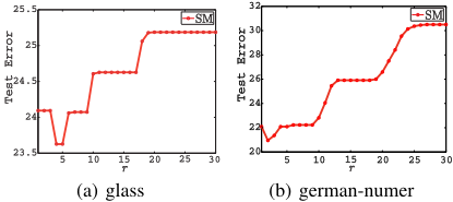
In the first experiment, we compare the performance of our proposed SM criterion with five popular kernel selection criteria: 5-fold cross-validation (CV), efficient leaveone-out cross-validation (ELOO) [Cawley, 2006], centered kernel target alignment (CKTA) [Cortes et al., 2010], feature space-based kernel matrix evaluation (FSM) [Nguyen and Ho, 2007] and the latest eigenvalue ratio (ER) [Liu and Liao, 2015]. For each data set, we choose the kernel parameter τ by each kernel selection criterion on the training set and then evaluate the test error for the chosen parameters on the test set. In this experiment, we set r = 3. We will explore the influence of r later. Table 2 reports the average test errors that can be summarized as follows: (a) SM is significantly better than FSM and CKTA on nearly all data sets. This can be explained by the fact that FSM and CKTA don't have theoretical guarantee for special learning algorithm, so the kernels chosen by these criteria can not guarantee good generalization performance; (b) SM is better than CV and ER on most data sets. In particular, SM is significantly better than ER (or CV) on 15 (or 11) of 25 data sets, but only 4 (or 5) sets significantly worse on the remaining data sets; (c) SM gives comparable results with ELOO. In particular, SM is significantly better than ELOO on 9 data sets (autos, breast-w, breast-cancer, hepatitis, ionosphere, labor, segment, vote and wdbc) and is significantly worse on 8 data sets (diabetes, glass, heart, pima, liver-disorders, sonar, wpbc and tic-tac-toe). The run time of SM, CV, ELOO, CKTA, FSM and ER are reported in Table 3. It turns out that SM is much faster than CV, ELOO and ER, and gives comparable results with CKTA and FSM. The above results manifest that SM can guarantee generalization performance and has high computational efficiency as well.
| SM | CV | ELOO | CKTA | FSM | ER | |
|---|---|---|---|---|---|---|
| a1a | 63.77 | 704.50 | 217.03 | 87.51 | 79.71 | 422.71 |
| a2a | 124.53 | 1995.76 | 810.87 | 172.28 | 156.68 | 1558.70 |
| anneal | 0.28 | 4.60 | 0.84 | 0.43 | 0.55 | 1.36 |
| australian | 8.30 | 111.31 | 30.33 | 11.34 | 9.51 | 52.53 |
| autos | 0.10 | 2.18 | 0.23 | 0.17 | 0.29 | 0.37 |
| breast-cancer | 8.05 | 104.55 | 27.13 | 11.10 | 9.36 | 47.68 |
| breast-w | 8.59 | 105.39 | 29.77 | 11.80 | 10.11 | 49.86 |
| colic | 1.55 | 25.72 | 6.52 | 2.15 | 2.17 | 11.60 |
| glass | 0.33 | 5.74 | 1.15 | 0.53 | 0.66 | 2.00 |
| heart | 1.02 | 14.71 | 3.66 | 1.12 | 1.20 | 6.33 |
| hepatitis | 0.38 | 6.55 | 1.42 | 0.58 | 0.70 | 2.44 |
| ionosphere | 1.59 | 24.60 | 6.08 | 2.03 | 2.06 | 10.60 |
| labor | 0.16 | 2.88 | 0.42 | 0.28 | 0.42 | 0.67 |
| pima | 10.99 | 137.19 | 36.60 | 15.11 | 12.74 | 62.45 |
| segment | 7.50 | 91.73 | 23.83 | 10.49 | 8.93 | 42.63 |
| diabetes | 10.70 | 134.71 | 36.26 | 14.90 | 12.51 | 62.46 |
| german.numer | 21.80 | 249.98 | 72.63 | 29.59 | 26.27 | 127.51 |
| liver-disorders | 1.37 | 21.04 | 5.46 | 1.91 | 1.94 | 9.27 |
| sonar | 0.62 | 10.53 | 2.34 | 0.87 | 0.98 | 4.06 |
| vehicle | 2.03 | 35.64 | 9.35 | 2.86 | 2.85 | 15.95 |
| vote | 2.03 | 34.43 | 9.33 | 2.79 | 2.81 | 15.92 |
| wpbc | 0.52 | 9.06 | 2.07 | 0.76 | 0.92 | 3.33 |
| bupa | 1.36 | 21.09 | 5.34 | 1.85 | 1.88 | 9.19 |
| tic-tac-toe | 18.93 | 224.13 | 63.10 | 26.13 | 23.04 | 107.12 |
| wdbc | 5.75 | 61.32 | 19.18 | 7.86 | 6.80 | 33.65 |
In the following experiment, we explore the influence of the parameter r of SM. Figure 1 plots the average test errors with different r (due to space limit, we randomly select 2 data sets). For each fixed r, we choose the kernel parameter τ by SM on the training set, and evaluate the test errors for the chosen parameters on test set. We find that the optimal r belong to [2, 5] on most data sets. And we can also find out that we can randomly set r = 2, r = 3 or r = 4 in practice without sacrificing accuracy.
6 Conclusion
In this paper, we define a new spectral measure of a kernel matrix, which can be effectively calculated in O(n2 ) time complexity. With the spectral measure, we can bound the generalization errors of LSSVM and SVM, and propose the kernel selection criterion by minimizing the derived generalization error bounds, of which the minimum graph cut and maximum mean discrepancy are two special cases. The high computational efficiency and theoretical guarantee of the spectral measure may bring a new perspective on designing kernel selection criterion using spectral analysis.
Appendix A: Proof of the Theorem 1
To prove Theorem 1, we first prove the following Lemma:
Lemma 1. If fS is the solution of LSSVM, then
Proof. Note that (fS(x1), . . . , fS(xn))T = Kα where α = [K+λI]-1y. Thus
Let (βi, ui) be the spectral decomposition of K, then we have
Since Tr(K) ≤ |K|1 = C, we know that βj C ≤ Tr(K) C ≤ 1. According to Equation (4), we have yTK[K+λI]-1y = ∑ni=1 βi/C βi/C+λ/C 〈y, ui〉2 ≥ ∑ni=1 βi/C 1+λ/C 〈y, ui〉2 . Note that λi = βi/|K|1 = βi/C, vi = ui, where (λi, vi) is the spectral decomposition of N, thus
From the assumption ϕ(λi) ≤ λi, Equations (3), (4) and (5), we have ∑ni=1 yifS(xi) ≥ ∑ni=1 ϕ(λi) 1+λ/C 〈y, vi〉2 , which completes the proof.
Theorem 3 (Theorem 8 [Gao and Zhou, 2013]). For any δ > 0, with probability at least 1 - δ over the random choice of sample S with size n ≥ 5, every f ∈ HK satisfies the following bound:
Proof of the Theorem 1. Note that PrS[yfS(x) ≤ θ] = 1n ∑ni=1 1[yifS(xi)-θ], where 1[t] = 1, if t < 0, otherwise 1[t] = 0. Thus, it is easy to verify that
From the assumption that HK ranges in [-1,1], we have 1 - yifS(xi) + θ > 0. Thus, by Equation (6), we have
According to Equation (7) and Equation (2), we have
Substituting Equation (8) to Theorem 3, we have
This completes the proof for Theorem 1.
Appendix B: Proof of the Theorem 2
Similar with the proof of the Theorem 1, we first prove the following lemma:
Lemma 2. If fS be the solution of SVM, then
where d =min{-1, 1- 1 2λ }.
Proof. Note that fS(x) = ∑ni=1 αiK(xi, x), where α is the solution of the dual form of SVM. Thus, we have
where ⊗ is the entrywise matrix product (also known as the Hadamard product). Note that
where ci = min{αi, 1} -max{αi, 1}. Note that 0 ≤ αi ≤ 1 2λ , so we can obtain that
From Equation (10), we have
Thus, we can obtain that yTK(y ⊗ α) ≥ dC + yTKy = dC + ∑i βi〈yi, ui〉2 = dC + C ∑i λi〈yi, vi〉2 ≥ dC+C ∑i ϕ(λi) · 〈yi, vi〉2 , where (βi, ui) is the spectral decomposition of K. This completes the proof.
Proof of Theorem 2. According to Lemma 2 and Equation (7), we can obtain that
Substituting Equation (11) to Theorem 3, it is easy to complete the proof.
Acknowledgments
This work is supported in part by the National Natural Science Foundation of China (No.61673293, No.61602467, No.61303056), and Excellent Talent Introduction, Institute of Information Engineering, CAS (Y7Z0111107), and Youth Innovation Promotion Association, CAS (No.2016146).
@inproceedings{ijcai2017p295,
  title     = {Efficient Kernel Selection via Spectral Analysis},
  author    = {Li, Jian and Liu, Yong and Lin, Hailun and Yue, Yinliang and Wang, Weiping},
  booktitle = {Proceedings of the Twenty-Sixth International Joint Conference on
               Artificial Intelligence, {IJCAI-17}},
  publisher = {International Joint Conferences on Artificial Intelligence Organization},
  editor    = {Carles Sierra},
  pages     = {2124--2130},
  year      = {2017},
  month     = {8},
  note      = {Main track},
  doi       = {10.24963/ijcai.2017/295},
  url       = {https://doi.org/10.24963/ijcai.2017/295},
}
TY - CPAPER TI - Efficient Kernel Selection via Spectral Analysis AU - Li, Jian AU - Liu, Yong AU - Lin, Hailun AU - Yue, Yinliang AU - Wang, Weiping T2 - Proceedings of the Twenty-Sixth International Joint Conference on Artificial Intelligence, IJCAI-17 PB - International Joint Conferences on Artificial Intelligence Organization PY - 2017 SP - 2124 EP - 2130 DO - 10.24963/ijcai.2017/295 UR - https://doi.org/10.24963/ijcai.2017/295 ER -Copied
Machine-readable versions of this paper, for tools and AI agents:





