
Constrained Bayesian Reinforcement Learning via Approximate Linear Programming
Proceedings of the Twenty-Sixth International Joint Conference on Artificial Intelligence. Main track. Pages 2088-2095.
https://doi.org/10.24963/ijcai.2017/290
Keywords
- Uncertainty in AI: Markov Decision Processes
- Planning and Scheduling: POMDPs
- Machine Learning: Reinforcement Learning
Abstract
In this paper, we consider the safe learning scenario where we need to restrict the exploratory behavior of a reinforcement learning agent. Specifically, we treat the problem as a form of Bayesian reinforcement learning in an environment that is modeled as a constrained MDP (CMDP) where the cost function penalizes undesirable situations. We propose a model-based Bayesian reinforcement learning (BRL) algorithm for such an environment, eliciting risk-sensitive exploration in a principled way. Our algorithm efficiently solves the constrained BRL problem by approximate linear programming, and generates a finite state controller in an off-line manner. We provide theoretical guarantees and demonstrate empirically that our approach outperforms the state of the art.
- [Altman, 1999] Eitan Altman. Constrained Markov Deci- sion Processes. Chapman and Hall, 1999.
- [Araya-López et al., 2012] Mauricio Araya-López, Vincent Thomas, and Olivier Buffet. Near-optimal BRL using op- timistic local transition. In Proceedings of the 29th Inter- national Conference on Machine Learning, pages 97-104, 2012.
- [Asmuth et al., 2009] John Asmuth, Lihong Li, Michael L. Littman, Ali Nouri, and David Wingate. A Bayesian sam- pling approach to exploration in reinforcement learning. In Proceedings of the Twenty-Fifth Conference on Uncer- tainty in Artificial Intelligence, pages 19-26, 2009.
- [Dearden et al., 1998] Richard Dearden, Nir Friedman, and Stuart Russell. Bayesian Q-learning. In Proceedings of the 15th National Conference on Artificial Intelligence, pages 761-768, 1998.
- [Dearden et al., 1999] Richard Dearden, Nir Friedman, and David Andre. Model based Bayesian exploration. In Pro- ceedings of the Fifteenth Conference on Uncertainty in Ar- tificial Intelligence, pages 150-159, 1999.
- [Duff, 2002] Michael O'Gordon Duff. Optimal learning: Computational procedures for Bayes-adaptive Markov de- cision processes. PhD thesis, University of Massachusetts Amherst, 2002.
- [García and Fernández, 2012] Javier García and Fernando Fernández. Safe exploration of state and action spaces in reinforcement learning. Journal of Artificial Intelligence Research, 45(1):515-564, 2012.
- [Hans et al., 2008] Alexander Hans, Daniel Schneega, An- ton M. Schäfer, and Steffen Udluft. Safe exploration for reinforcement learning. In Proceedings of the European Symposium on Artificial Neural Network, pages 143-148, 2008.
- [Howard and Matheson, 1972] Ronald A. Howard and James E. Matheson. Risk-sensitive markov decision processes. Management Science, 18(7):356-369, 1972.
- [Hsu et al., 2007] David Hsu, Wee Sun Lee, and Nan Rong. What makes some POMDP problems easy to approxi- mate? In Advances in Neural Information Processing Sys- tems 20, pages 689-696, 2007.
- [Iyengar, 2005] Garud N. Iyengar. Robust dynamic program- ming. Mathematics of Operations Research, 30(2):257- 280, 2005.
- [Kim et al., 2011] Dongho Kim, Jaesong Lee, Kee-Eung Kim, and Pascal Poupart. Point-based value iteration for constrained pomdps. In Proceedings of the Twenty-Second International Joint Conference on Artificial Intelligence, pages 1968-1974, 2011. IJCAI
- [Kim et al., 2012] Dongho Kim, Kee-Eung Kim, and Pascal Poupart. Cost-sensitive exploration in Bayesian reinforce- ment learning. In Advances in Neural Information Pro- cessing Systems 25, pages 3068-3076, 2012.
- [Kolter and Ng, 2009] J. Zico Kolter and Andrew Y. Ng. Near-Bayesian exploration in polynomial time. In Pro- ceedings of the 26th Annual International Conference on Machine Learning, pages 513-520, 2009.
- [Mihatsch and Neuneier, 2002] Oliver Mihatsch and Ralph Neuneier. Risk-sensitive reinforcement learning. Machine Learning, 49(2):267-290, 2002.
- [Minka, 1998] Thomas P. Minka. Bayesian linear regression. Technical report, Microsoft research, 1998.
- [Nilim and El Ghaoui, 2005] Arnab Nilim and Laurent El Ghaoui. Robust control of Markov decision processes with uncertain transition matrices. Operations Research, 53(5):780-798, 2005.
- [Poupart et al., 2006] Pascal Poupart, Nikos Vlassis, Jesse Hoey, and Kevin Regan. An analytic solution to dis- crete Bayesian reinforcement learning. In Proceedings of the 23rd International Conference on Machine Learning, pages 697-704, 2006.
- [Poupart et al., 2015] Pascal Poupart, Aarti Malhotra, Pei Pei, Kee-Eung Kim, Bongseok Goh, and Michael Bowl- ing. Approximate linear programming for constrained par- tially observable Markov decision processes. In Proceed- ings of the Twenty-Ninth AAAI Conference on Artificial In- telligence, pages 3342-3348, 2015.
- [Strens, 2000] Malcolm J. A. Strens. A Bayesian framework for reinforcement learning. In Proceedings of the Sev- enteenth International Conference on Machine Learning, pages 943-950, 2000.
- [Sutton and Barto, 1998] Richard S. Sutton and Andrew G. Barto. Reinforcement Learning: An Introduction. MIT Press, 1998.
- [Tziortziotis et al., 2013] Nikolaos Tziortziotis, Chris- tos Dimitrakakis, and Konstantinos Blekas. Linear Bayesian reinforcement learning. In Proceedings of the Twenty-Third International Joint Conference on Artificial Intelligence, 2013. IJCAI
References were extracted automatically from the PDF and may contain errors.
Full text extracted automatically from the PDF; figures, tables and equations may differ. The PDF is the version of record.
1 Introduction
In reinforcement learning (RL), the agent interacts with the unknown environment to maximize the long-term return defined by real-valued reward signals [Sutton and Barto, 1998]. Due to the uncertain nature of the environment, the agent faces an exploration-exploitation trade-off, a fundamental challenge in RL: the agent has to weigh between the action that yields the best return based on past experience and other actions that facilitate new experiences towards discovering better actions. This paper considers model-based Bayesian reinforcement learning (BRL) [Dearden et al., 1999; Duff, 2002; Poupart et al., 2006], which provides a principled way of optimally balancing between exploration and exploitation in the Bayesian perspective, with the goal of obtaining sample-efficient learning behaviours.
Still, in many situations, the notion of safety or risk avoidance is crucial and should be considered as another prime objective to the RL agent [Mihatsch and Neuneier, 2002; Hans et al., 2008; Garc´ıa and Fern´andez, 2012]. For example, a Mars rover has to reach a target position as fast as possible, but at the same time, it should avoid navigating into dangerous ditches, which can potentially render it irrecoverable.
∗This work was partly supported by Institute for Information & communications Technology Promotion(IITP) grant funded by the Korea government(MSIP) (No.2014-0-00147, Basic Software Research in Human-level Lifelong Machine Learning (Machine Learning Center)) and was conducted at High-Speed Vehicle Research Center of KAIST with the support of Defense Acquisition Program Administration (DAPA) and Agency for Defense Development (ADD).
This safe behavior requirement has been captured in various forms, mostly considering the risk of performing very poorly due to the inherent stochasticity of the environment. In this formulation, the classic objective of maximizing expected return may be modified to minimize the variance of returns [Howard and Matheson, 1972], or to maximize the return in the worst case [Iyengar, 2005; Nilim and El Ghaoui, 2005].
In this paper, we consider the constrained MDP (CMDP) [Altman, 1999] as the framework for modeling the safe exploration requirement. CMDP assumes that actions incur costs as well as rewards, where the goal is to obtain a behaviour policy that maximizes the expected cumulative rewards while the expected cumulative costs are bounded. Under these circumstances we can naturally encode the risks of specific behaviours as cost functions and the degree of risk taking as cost constraints respectively. Here, we assume that the reward functions and the cost functions are known to the RL agent and only the transition probabilities are unknown, as in many model-based BRL studies [Poupart et al., 2006; Asmuth et al., 2009; Kolter and Ng, 2009; Araya-L´opez et al., 2012; Kim et al., 2012]. Specifically, following [Kim et al., 2012], we model BRL as a planning problem with the hyperstate constrained partially observable MDP (CPOMDP) [Kim et al., 2011] and adopt constrained approximate linear programming (CALP) [Poupart et al., 2015] to compute Bayesoptimal policies in an off-line manner.
Most of the successful approximate planning algorithms for (constrained) POMDPs confine the whole set of infinitely many beliefs to a finite set. This technique was also adopted in CALP [Poupart et al., 2015] to treat other beliefs as convex combinations of finite samples of beliefs. However, doing so for model-based BRL can be problematic as it is not straightforward to represent a distribution over the transition probabilities as a finite convex combination. As will be described in the later part of the paper, one of our contributions is in introducing the notion of 'slip to ϵ-close beliefs', which enables a theoretical analysis and provides empirical support.
2 Background
We model the environment as a constrained Markov decision process (CMDP), defined by a tuple 〈S,A, T,R,C = {Ck}1..K, c = {ck}1..K, γ, s0〉 where S is the set of states s, A is the set of actions a, T(s′ |s, a) = Pr(s′ |s, a) is the transition probability, R(s, a) ∈ R is the reward function which denotes immediate reward incurred by taking action a in state s, Ck(s, a) ∈ R is the kth cost function upper bounded by ck ∈ R of kth cost constraint, γ ∈ [0, 1) is the discount factor, and s0 is the initial state. The goal is to compute an optimal policy π∗ that maximizes expected cumulative rewards while expected cumulative costs are bounded.
The optimal policy of a CMDP is generally stochastic and can be obtained by solving the following linear program (LP) [Altman, 1999].
where y(s, a) can be interpreted as a discounted occupancy measure of (s, a), and δ(x, y) is a Dirac delta function that has a value of 1 if x = y and 0 otherwise. Once the optimal solution y(s, a) is obtained, an optimal stochastic policy and the corresponding optimal value are computed as π∗ (a|s) = Pr(a|s) = y(s, a)/ ∑a′ y(s, a′ ) and V ∗ R (s0) = ∑s,a R(s, a)y(s, a) respectively.
The constrained partially observable Markov decision process (CPOMDP) generalizes the CMDP by allowing partial observability and is defined by the tuple 〈S,A,O, T,Z,R,C, c, γ, b0〉. Additional components are O, Z, and b0, where O is the set of observations o and Z(o|s′ , a) = Pr(o|s′ , a) is the observation probability of observing o when taking action a and moving to state s′ , and b0(s) = Pr(s0 = s) is the initial belief at time step 0, respectively. Since the current Markovian state is not directly observable, the agent infers a belief bt(s) = Pr(st = s) (which is a sufficient statistic for decision making) at every time step using the Bayes rule: upon executing a in b and observing o, the updated belief bao is
Consequently, decision making in CPOMDPs can be understood as a process of repeating: 1) choose an action based on the current belief, 2) update the current belief distribution based on the last action and observation using Eq. (2). A CPOMDP is equivalent to a constrained belief state CMDP 〈 ¯ S,A, ¯ T, ¯R, ¯C, c, γ, ¯ s0〉. Here ¯ s0 = b0 and ¯ S = B is the set of reachable beliefs starting from b0. Transition probability ¯ T(b′ |b, a) is constructed from components of the original CPOMDP and is expressed in terms of beliefs.
Similarly, the reward and cost functions are represented as
Although the resulting constrained belief MDP can be solved by LP (1) in principle, the cardinality of B is usually very large or even infinite, which makes the problem computationally intractable. To tackle the intractability, several approximate algorithms have been proposed, such as CPBVI, which is based on dynamic programming [Kim et al., 2011], and CALP, which is based on linear programming [Poupart et al., 2015]. CALP has been shown to perform much better than CPBVI.
3 Constrained BRL via Approximate Linear Programming
In many practical situations, too much exploration can severely impact an RL agent and therefore exploration should be restricted. Restrictions can naturally be encoded as constraints on cost functions that quantify the impact of certain behaviours. In this section, we propose a model-based BRL algorithm for the CMDP environment, leading to costsensitive exploration in a principled way. To this end, we will take the following approach: we first convert the constrained BRL problem into a hyper-state CPOMDP planning problem. The CPOMDP planning problem is then cast into an equivalent belief-state CMDP planning problem. Finally, we use constrained approximate linear programming (CALP) to efficiently compute the Bayes-optimal policy in an offline manner. These steps are explained in subsequent subsections.
3.1 Constrained BRL as CPOMDP Planning
Model-based BRL computes a full posterior distribution over the transition models and use it to make decisions. We can formulate model-based BRL in a CMDP environment 〈S,A, T,R,C, c, γ, s0〉 as a hyper-state CPOMDP planning problem [Duff, 2002; Poupart et al., 2006; Kim et al., 2012], which is formally defined by the tuple 〈S+,A,O+, T +,Z +,R+,C+, c, γ, b+0 〉. Assuming finite state and action spaces, each component is specifically S+ = S × {θsas′ }, O+ = S, T +(〈s′ , θ′ 〉|〈s, θ〉, a) = θsas′ δ(θ, θ′ ),
A belief distribution over S+ in a hyper-state CPOMDP is a pair (s, b) consisting of a Markovian state s of the original CMDP and the posterior distribution b(θ) over unknown parameters θ. Here b(θ) is commonly chosen to be a product of Dirichlet distributions since Dirichlets are conjugate priors of the multinomial transition probabilities:
When the agent in belief (¯ s, b) takes an action ¯a and observes the successor state ¯ s′ , the belief is updated to (¯ s′ , b′ ), where b′ is defined as:
where η is a normalizing constant. The hyper-state CPOMDP can also be easily understood as an equivalent belief-state CMDP 〈 ¯ S+,A, ¯ T +, ¯R+, ¯C+, c, γ, ¯ s+0 〉. Here ¯ S+ = S × B and ¯ s+0 = (s0, b0) where B is the set of possible posterior distributions over θsas′ from initial prior b0. Transition probabilities among belief states (s, b) are defined as
Similarly, the reward function and the cost functions are
In theory, this belief-state CMDP can be solved using the following LP, which is an extension of (1) and the one in [Poupart et al., 2015] to treat hyper belief states:
3.2 Approximate Linear Programming
The main challenge in solving the linear program (8) lies in the fact that the number of beliefs |S×B| is infinite, yielding infinitely many variables and constraints in the LP. We thus approximate (8) using finitely sampled beliefs. In order to facilitate a formal analysis, we assume a finite set of beliefs ̂ B ⊂ B that covers the entire belief space fairly well. More formally, we assume that there exists a constant ϵ such that
where ‖·‖1 denotes total variance distance
Since ̂ B does not completely cover B for ϵ > 0, we need to re-define the transition function T(s′ , b′ |s, b, a) among (s, b) and (s′ , b′ ) ∈ S × ̂ B. From the original, exact transition probability T (s′ , b′ |s, b, a) defined over (s, b) ∈ S × B:
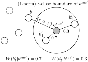
we relax δ(b′ , bsas′ ) to W(b′ |bsas′ ) that has non-zero probability only for ϵ-close beliefs:
where W is defined as a probability distribution over ̂ B.
where κ is the normalizing constant ∑b′∈ ̂ B W(b′ |bsas′ ) = 1 and K(b, b′ ) ≥ 0 is a similarity measure between two beliefs b(θ) and b′ (θ). This relaxation can be interpreted as "slipping" to one of the ϵ-close successor beliefs with probability W. Figure 1 depicts the construction process of W. Thus, we approximate the original LP (8) by using a finite set of beliefs ̂ B and replacing T by ̂ T. Algorithm 1 describes the overall process of computing the approximate Bayes-optimal policy.
The policy (π, W ) obtained from Algorithm 1 constitutes a finite state controller with |S|| ̂ B| nodes and is executed in the real environment as follows: the initial node of the controller is set to (s0, b0). At every time step, sample an action a ∼ π(a|s, b) based on the current node (s, b) for execution. Then, observe the next state s′ from the environment and sample b′ ∼ W(b′ |bsas′ ). Finally, the new node of the controller is set to (s′ , b′ ) and repeat.
Algorithm 1 Constrained BRL via Approximate LP
B, b0.
Input: S,A,R,C, c, γ, s0, ̂
B, and a ∈ A do
Compute W(b′ |bsas′ ) ∀b′ by Eq (11)
for each s, s′ ∈ S, b ∈ ̂
end for
̂
T(s′ , b′ |s, b, a) ←Eb[θsas′ ] · W(b′ |bsas′ ) ∀s, b, a, b, b′
y ← solve LP (8) with ̂
T (s′ , b′ |s, b, a)
B and ̂
B, and a ∈ A do
π(a|s, b) ← y(s, b, a)/ ∑a′ y(s, b, a′ )
for each s ∈ S, b ∈ ̂
end for
Output: (π,W): finite state controller, ̂ V ∗ R (s0, b0): approximate Bayes-optimal value
We remark that Poupart et al. [2015] take a similar approach to solving CPOMDPs by considering finitely sampled beliefs. Specifically, they approximate the transitions by relaxing δ(b′ , bao ) in (3) as interpolation weights w(b′ , bao ) such that ∑b′∈̂ B w(b′ , bao )b′ = bao , ∑b′∈̂ B w(b′ , bao ) = 1 and w(b′ , bao ) ≥ 0. This approach cannot be directly adopted in the Bayesian learning setting since a belief is no longer a finite-dimensional probability vector but rather a probability density function. There is no straightforward way to approximate an arbitrary Dirichlet using a convex combination of finitely many Dirichlets.
4 Theoretical Analysis
In this section, we provide a formal analysis of the error bound incurred by taking a finite set of beliefs and using the 'slip to ϵ-close belief' approximation scheme to re-define the transition probabilities. In order to facilitate our analysis, we first show the result on the single objective case, i.e. rewardonly POMDPs.
Lemma 1. Suppose that the reward function is bounded in [-Rmax, Rmax]. For any b,̂b ∈ B such that ‖b-̂b‖1 ≤ ϵ, the following inequality holds.
Proof. It is well known that the optimal value of POMDP is piecewise linear and convex function, and can be expressed as an inner product between a belief distribution b and a set of alpha functions Γ∗ = {α1, · · · , α|Γ|}.
Note that this lemma is same as lemma 1 in [Hsu et al., 2007] with a simpler proof.
Lemma 2. Suppose that for all b ∈ B, there exists ̂b ∈ ̂ B such that ‖b -̂b‖1 ≤ ϵ. Let H be an exact value-function mapping, and ̂H be a value-function mapping of approximate POMDP with 'slip to ϵ-close belief ' approximation. Suppose that V ∗ is an unique fixed point solution of HV = V . Then, the following inequality holds:
where ϵ1 is defined in Lemma 1.
Proof. For any s ∈ S, b ∈ ̂ B, a ∈ A, and s′ ∈ S,
(Lemma 1)
Therefore, for any s ∈ S and b ∈ ̂ B,
Similarly, we can obtain:
As a consequence, we get the result ‖HV ∗ - ̂HV ∗ ‖ ≤ γϵ1.
Theorem 1. Suppose that the reward function is bounded in [-Rmax,Rmax], and for all b ∈ B, there exists ̂b ∈ ̂ B such that ‖b -̂b‖1 ≤ ϵ. Let V ∗ be the fixed point solution V ∗ = HV ∗ (optimal value function of original POMDP), and ̂ V ∗ be the fixed point solution ̂ V ∗ = ̂Ĥ V ∗ (optimal value function of approximate POMDP with 'slip to ϵ-close belief ' approximation). Then, the following inequality holds.
Proof.
In the above, ̂H denotes the approximate Bellman backup that arises from finitely sampled beliefs ̂ B and 'slip to ϵ-close belief' transition approximation scheme.
Unfortunately, this result cannot be naively extended to constrained POMDPs. To make the connection between single objective POMDPs and constrained POMDPs, we should look at the dual form of the LP in (8) given by:
If we fix λ in the above formulation, the problem becomes the single objective POMDP with new reward function R(s, a) - λ⊤C(s, a). The solution can be obtained through the dynamic programming with the backup operator Hλ defined as:
which is a contraction mapping and has an unique fixed point solution V ∗λ. Then, the LP dual problem can be reduced to minλ [V ∗λ(s0, b0) +λ⊤c]. Moreover, if there is an optimal solution y∗ to primal LP, there must exist the corresponding dual optimal solution V ∗ and λ∗ , and duality gap is zero (i.e. V ∗ R (s0, b0, c) = V ∗λ∗(s0, b0) + λ∗⊤c) by the strong duality theorem. We can now apply the result in Theorem 1 with a fixed λ since V ∗λ is a value function of single objective POMDP.
Lemma 3. Suppose that reward function and cost functions of the CMDP environment are bounded in [0,Rmax] and [0,Cmax] respectively. Let V ∗λ be the optimal value function of the POMDP with reward function of R(s, a) - λ⊤C(s, a) and ̂ V ∗λ be the optimal value of the approximate POMDP with the same reward function and 'slip to ϵ-close belief' approximation. Then, the following inequality holds for all λ ≥ 0:
Therefore, by simply applying Theorem 1 with the reward range of [-Rmax - ‖λ‖1Cmax, Rmax + ‖λ‖1Cmax], we get the result.
Lemma 3 indicates that the approximation error can depend on the magnitude of λ, and the following Lemma 4 shows that ‖λ‖1 can be bounded.
Lemma 4. Suppose that reward function is bounded in [0,Rmax] and there exists τ > 0 and policy π such that V π C (s0, b0) + τ1 ≤ c. Then, the following inequality holds:
Proof. Let C = {c | there exists a policy π such that V π C (s0, b0) ≤ c}. For any c, c′ ∈ C,
where λ′∗ = argminλ′ [V ∗λ′(s0, b0) + λ′⊤c′ ], and λ∗ = argminλ[V ∗λ(s0, b0) + λ⊤c]. For any τ > 0 such that c- τ1 ∈ C, let c′ = c- τ1. Then,
Remark. Intuitively, τ represents how much we can reduce the cost constraint without making the problem infeasible. For example, when the cost constraint c is set to 100, while the minimum cost value of the given CMDP environment is 30 (i.e. minπ V π C (s0, b0) = 30), τ = 100 - 30 = 70.
We can now show the main result that bounds the error in the value function due to approximate LP:
Theorem 2. Suppose that reward function and cost functions of CMDP environment are bounded in [0,Rmax] and [0,Cmax] respectively. Let V ∗ R (s0, b0, c) be an optimal value of the original CPOMDP with cost constraint c, and ̂ V ∗ R (s0, b0, c) be an optimal value function of approximate CPOMDP with cost constraint c and 'slip to ϵ-close beliefs' approximation. Then, the following inequality holds:
Proof.
5 Experiments
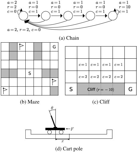
We conducted experiments on 3 discrete state domains and 1 continuous state domain depicted in Figure 2. The chain domain [Dearden et al., 1998] has 5 states and 2 actions. The agent receives large reward of 10 by executing action 1 at the fifth state, and small of 2 by executing action 2 at any state. With probability 0.2 agent slips, which means that the opposite transition occurs. We prepared a constrained version of this domain by allocating cost 1 for action 1 and cost 0 for action 2, which makes the excessively taking action 1 may violate the cost constraint, following [Kim et al., 2012]. The maze domain [Strens, 2000] has 33 rooms and three flags. There are 5 actions {left, right, up, down, stay} that allow moving to neighboring rooms. Every action except for stay fails with probability 0.1. If an action fails, the agent randomly slips into one of the directions orthogonal to the intended one. The reward is given by the number of captured flags when the agent arrives at the goal. Since there are 33 rooms and 8 possible status of captured flags, there are 264 states in total. We defined the cost 1 to every action except staying at the starting cell. The cliff domain [Sutton and Barto, 1998] has 24 states and 4 actions {left, right, up, down}. Every action fails with probability 0.1. If an action fails, the agent randomly slips into one of the not intended directions. The agent receives large reward of 20 once reaching the goal state, and reward of -10 when it falls into cliff. We assign cost of 2 to the cliff and the locations one unit away from the cliff (high-risk area) and cost of 1 to the locations two units away from the cliff (medium-risk area) and cost of 0 elsewhere (low-risk area). The cart pole [Sutton and Barto, 1998] domain is the classical control problem to keep the pole upright. The state is encoded s = [x, ˙x, θ, ˙ θ], where x is the position, ˙x is the velocity, θ is the angle, and ˙ θ is the angular velocity. There are two actions {left, right} that apply a force of -1 or +1 to the cart. A reward of -1 is received if the cart or pole is out of the range: |x| ≥ 2.4 or |θ| ≥ 12◦ . Cost function is defined by C(s, a) = |x| to encourage the agent to stay in the middle.
5.1 Experimental Setup
Finite State Domains
For all the finite state domains, we used two kinds of structural priors, "tied" and "semi". In both tied and semi, it is assumed that the transition dynamics are known except for the slip probabilities. The tied prior assumes that the slip probability is independent of state and action, so there is only one unknown parameter. The semi prior assumes actiondependent slip probabilities, so the number of unknown parameters is 2 for chain, 5 for maze, and 4 for cliff, respectively. We used uninformative Dirichlet priors. Approximate transitions in (10) were constructed by
where σ is set to 0.5. ̂ B were collected by uniformly random policy executed in the environment for 50 time steps.
In the chain and cliff domains, we report the results of 200 trials of the first 2000 times steps with discount factor γ = 0.99. In the maze domain, we report the results of 100 tirals of the first 1000 time steps with discount factor γ = 0.95.
Continuous State Domain
In cart pole, the environment dynamics are modeled as a linear dynamical system, as in [Tziortziotis et al., 2013].
Here φ(s) = [s, 1]⊤ and the transition model is parameterized by {(Aa, Va)}∀a. We use matrix-normal prior for A and inverse-Wishart prior for V . Given the samples
| domain | c | algorithm | avg discounted total reward | avg discounted total cost | time (min) |
|---|---|---|---|---|---|
| chain-tied | 100 | CBEETLE CBRL-ALP | 355.85±4.55 339.77±8.01 | 99.64±0.08 91.26±2.44 | 1.2 0.1 |
| 75 | CBEETLE CBRL-ALP | 305.02±3.82 315.22±7.14 | 74.96±0.04 71.46±1.75 | 2.1 0.1 | |
| 50 | CBEETLE CBRL-ALP | 243.54±3.29 289.86±6.25 | 50.03±0.10 48.37±1.10 | 9.7 0.1 | |
| 25 | CBEETLE CBRL-ALP | 218.54±1.94 235.06±6.03 | 25.03±0.04 23.72±1.12 | 34.8 0.1 | |
| chain-semi | 100 | CBEETLE CBRL-ALP | 355.12±4.16 327.10±8.91 | 98.42±0.14 83.51±3.39 | 1.9 0.2 |
| 75 | CBEETLE CBRL-ALP | 298.03±4.09 307.22±7.87 | 75.00±0.05 66.19±2.42 | 3.8 0.2 | |
| 50 | CBEETLE CBRL-ALP | 237.71±3.49 276.01±7.65 | 50.10±0.10 44.36±1.89 | 16.7 0.2 | |
| 25 | CBEETLE CBRL-ALP | 214.08±2.14 226.74±6.32 | 24.94±0.06 22.07±1.73 | 89.9 0.2 | |
| maze-tied | 20 | CBEETLE(∗) CBRL-ALP | 1.02±0.02 1.03±0.02 | 19.04±0.02 19.09±0.03 | 242.5 39.3 |
| 18 | CBEETLE(∗) CBRL-ALP | 0.93±0.04 0.96±0.02 | 17.96±0.46 17.92±0.22 | 733.1 41.0 | |
| cliff-tied | 100 | CBEETLE CBRL-ALP | 121.21±4.94 166.20±2.32 | 91.88±0.54 64.75±3.57 | 173.8 1.5 |
| 50 | CBEETLE CBRL-ALP | 52.98±3.77 160.89±1.57 | 44.41±0.50 44.72±0.90 | 180.0 1.5 | |
| 30 | CBEETLE CBRL-ALP | -104.52±4.58 150.19±1.41 | 54.64±0.97 25.99±0.83 | 206.8 1.5 | |
| cliff-semi | 100 | CBEETLE CBRL-ALP | 51.55±5.57 161.05±1.88 | 91.25±0.63 51.65±2.81 | 485.0 7.9 |
| 50 | CBEETLE CBRL-ALP | -78.80±5.89 158.44±1.59 | 63.03±0.73 42.28±1.00 | 594.7 7.9 | |
| 30 | CBEETLE CBRL-ALP | -117.80±9.29 146.91±1.39 | 43.09±1.28 22.44±0.86 | 657.4 7.9 |
{(st, at, st+1)}t=1..N, the posteriors can be obtained in a closed form [Minka, 1998].
To construct finite set of beliefs ̂ S× ̂ B, we collected 10000 states by taking random actions and quantized them into 256 representative states via K-means clustering, which constitutes ̂ S. Then, ̂ B was constructed by gathering beliefs during the first 100 steps at every 10 step-interval. Pr(s′ |s, b, a) in (10) was replaced by
which is proportional to the posterior predictive distribution. W(b′ |bsas′ ) was defined by (13) with σ = 1. The results are averaged over 100 trials of the first 10000 steps with discount factor γ = 0.99.
5.2 Results
Table 1 summarizes the experimental results for discrete domains, comparing our algorithm CBRL-ALP to the previous state-of-the-art approach CBEETLE [Kim et al., 2012]. Overall, our method outperforms in computation speed by an order of magnitude, while yielding good policies. In addition, CBEETLE generally slowed down as c became tighter, but CBRL-ALP was barely affected by the cost constraint. Note that our algorithm (and CBEETLE) generally achieves lower average total reward in the semi prior compared to the tied prior. This is a natural result since the agent has more uncertainty (more unknown parameters) regarding the dynamics and as such, it has to act more conservatively to meet the cost constraint.
| c | avg discounted total reward | avg discounted total cost | ̂ V ∗ C (s0, b0) |
|---|---|---|---|
| 50 | -0.51 ±0.11 | 30.18 ±3.01 | 49.48 ±0.26 |
| 40 | -1.12 ±0.28 | 15.99 ±2.05 | 40.00 ±0.00 |
| 30 | -3.19 ±0.48 | 7.03 ±0.68 | 30.00 ±0.00 |
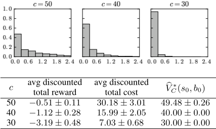
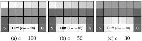
Figure 3 depicts the risk-sensitive behaviour in the cliff domain, where the darkness mark the visitation frequency of each state. When c = 100 (weakly constrained), agent tries to reach the goal as fast as possible to maximize rewards. As we lower c, it starts to trade-off between reward and cost, making the agent take a detour to be safer.
Figure 4 summarizes the experimental result of the cart pole domain. As we lower c, the agent start to trade-off reward for cost, which makes the agent be more forced to stay in the middle by tolerating the fall downs. We can also see from the table that the total cost estimated by the algorithm mathces c. As for the computation time, it took 105 minutes to construct ̂ T (s′ , b′ |s, b, a) and 0.3 minute to solve the LP on a single CPU machine. We remark that most of the computation time is spent on computing the transition probabilies, which should be easily parallelizable using GPUs.
6 Conclusion and Future work
In this paper, we presented CBRL-ALP, a model-based BRL algorithm in CMDP environment to deal with the safe exploration in a principled way. We showed that the constrained BRL problem can be solved efficiently via approximate linear programming. Our theoretical analysis shows that the algorithm computes approximate Bayes-optimal value functions and the approximation error can be bounded by the coverage of sampled beliefs. Experimental results show the cost-sensitive behaviours and effectiveness of our algorithms empirically, outperforming the previous state-of-the-art approach, CBEETLE by orders of magnitude in computation time.
As for the future work, we plan to focus on developing scalable algorithm that can be applied to more challenging domains. Extension to online version of the algorithm or application of function approximation would be promising.
@inproceedings{ijcai2017p290,
  title     = {Constrained Bayesian Reinforcement Learning via Approximate Linear Programming},
  author    = {Lee, Jongmin and Jang, Youngsoo and Poupart, Pascal and Kim, Kee-Eung},
  booktitle = {Proceedings of the Twenty-Sixth International Joint Conference on
               Artificial Intelligence, {IJCAI-17}},
  publisher = {International Joint Conferences on Artificial Intelligence Organization},
  editor    = {Carles Sierra},
  pages     = {2088--2095},
  year      = {2017},
  month     = {8},
  note      = {Main track},
  doi       = {10.24963/ijcai.2017/290},
  url       = {https://doi.org/10.24963/ijcai.2017/290},
}
TY - CPAPER TI - Constrained Bayesian Reinforcement Learning via Approximate Linear Programming AU - Lee, Jongmin AU - Jang, Youngsoo AU - Poupart, Pascal AU - Kim, Kee-Eung T2 - Proceedings of the Twenty-Sixth International Joint Conference on Artificial Intelligence, IJCAI-17 PB - International Joint Conferences on Artificial Intelligence Organization PY - 2017 SP - 2088 EP - 2095 DO - 10.24963/ijcai.2017/290 UR - https://doi.org/10.24963/ijcai.2017/290 ER -Copied
Machine-readable versions of this paper, for tools and AI agents:





