
Semi-supervised Feature Selection via Rescaled Linear Regression
Proceedings of the Twenty-Sixth International Joint Conference on Artificial Intelligence. Main track. Pages 1525-1531.
https://doi.org/10.24963/ijcai.2017/211
Keywords
- Machine Learning: Machine Learning
- Machine Learning: Feature Selection/Construction
Abstract
With the rapid increase of complex and high-dimensional sparse data, demands for new methods to select features by exploiting both labeled and unlabeled data have increased. Least regression based feature selection methods usually learn a projection matrix and evaluate the importances of features using the projection matrix, which is lack of theoretical explanation. Moreover, these methods cannot find both global and sparse solution of the projection matrix. In this paper, we propose a novel semi-supervised feature selection method which can learn both global and sparse solution of the projection matrix. The new method extends the least square regression model by rescaling the regression coefficients in the least square regression with a set of scale factors, which are used for ranking the features. It has shown that the new model can learn global and sparse solution. Moreover, the introduction of scale factors provides a theoretical explanation for why we can use the projection matrix to rank the features. A simple yet effective algorithm with proved convergence is proposed to optimize the new model. Experimental results on eight real-life data sets show the superiority of the method.
- [Cai et al., 2010] Deng Cai, Chiyuan Zhang, and Xiaofei He. Unsupervised feature selection for multi-cluster data. In ACM SIGKDD International Conference on Knowledge Discovery and Data Mining, pages 333-342, 2010.
- [Chang et al., 2014] Xiaojun Chang, Feiping Nie, Yi Yang, and Heng Huang. A convex formulation for semi- supervised multi-label feature selection. In Twenty-Eighth AAAI Conference on Artificial Intelligence, pages 1171- 1177, 2014.
- [Cristianini and Shawe-Taylor, 2000] Nello Cristianini and John Shawe-Taylor. An Introduction to Support Vector Machines: And Other Kernel-based Learning Methods. Cambridge University Press, New York, NY, USA, 2000.
- [Doquire and Verleysen, 2013] Gauthier Doquire and Michel Verleysen. A graph laplacian based approach to semi-supervised feature selection for regression problems. Neurocomputing, 121:5-13, 2013.
- [Guyon and Elisseef, 2003] Isabelle Guyon and André Elis- seef. An introduction to variable and feature selection. Journal of Machine Learning Research, 3:1157-1182, 2003.
- [He et al., 2005] Xiaofei He, Deng Cai, and Partha Niyogi. Laplacian score for feature selection. In Advances in neu- ral information processing systems, pages 507-514, 2005.
- [Huang, 2015] Samuel H Huang. Supervised feature selec- tion: A tutorial. Artificial Intelligence Research, 4(2):22, 2015.
- [Kira and Rendell, 1992] Kenji Kira and Larry A. Rendell. A practical approach to feature selection. In The ninth inter- national workshop on Machine learning, pages 249-256, 1992.
- [Kong and Yu, 2010] Xiangnan Kong and Philip S Yu. Semi- supervised feature selection for graph classification. In Proceedings of the 16th ACM SIGKDD international con- ference on Knowledge discovery and data mining, pages 793-802. ACM, 2010.
- [Kononenko, 1994] Igor Kononenko. Estimating attributes: Analysis and extensions of relief. In Proceedings of ECML-94, pages 171-182, Italy, 1994. Springer Berlin Heidelberg.
- [Liu and Yu, 2005] Huan Liu and Lei Yu. Toward integrating feature selection algorithms for classification and cluster- ing. IEEE Transactions on Knowledge and Data Engineer- ing, 17(4):491-502, 2005.
- [Luo et al., 2013] Yong Luo, Dacheng Tao, Chang Xu, Dongchen Li, and Chao Xu. Vector-valued multi-view semi-supervised learning for multi-label image classifica- tion. In Proceedings of the Twenty-Seventh AAAI Confer- ence on Artificial Intelligence, AAAI'13, pages 647-653. AAAI Press, 2013.
- [Nie et al., 2010] Feiping Nie, Heng Huang, Xiao Cai, and Chris H Ding. Efficient and robust feature selection via joint ℓ 2,1 -norms minimization. In Advances in neural in- formation processing systems, pages 1813-1821, 2010.
- [Ren et al., 2008] Jiangtao Ren, Zhengyuan Qiu, Wei Fan, Hong Cheng, and Philip S. Yu. Forward semi-supervised feature selection. In Proceedings of the 12th Pacific-Asia Conference in Knowledge Discovery and Data Mining, pages 970-976, Berlin, Heidelberg, 2008. Springer Berlin Heidelberg.
- [Richard et al., 2010] D. Richard, P. E. Hart, and D. G Stork. Pattern classification. Wiley-Interscience, 2010.
- [Shi et al., 2014] Lei Shi, Liang Du, and Yi-Dong Shen. Ro- bust spectral learning for unsupervised feature selection. In IEEE International Conference on Data Mining, pages 977-982, Dec 2014.
- [Strutz, 2010] Tilo Strutz. Data fitting and uncertainty: A practical introduction to weighted least squares and be- yond. Vieweg and Teubner, Germany, 2010.
- [Wang et al., 2015] D. Wang, F. Nie, and H. Huang. Feature selection via global redundancy minimization. IEEE Transactions on Knowledge and Data Engineering, 27(10):2743-2755, Oct 2015.
- [Wold et al., 1984] Svante Wold, Arnold Ruhe, Herman Wold, and WJ Dunn, III. The collinearity problem in lin- ear regression. the partial least squares (pls) approach to generalized inverses. SIAM Journal on Scientific and Sta- tistical Computing, 5(3):735-743, 1984.
- [Xiang et al., 2012] Shiming Xiang, Feiping Nie, Gaofeng Meng, Chunhong Pan, and Changshui Zhang. Discrimi- native least squares regression for multiclass classification and feature selection. IEEE transactions on neural net- works and learning systems, 23(11):1738-1754, 2012.
- [Xu et al., 2010] Zenglin Xu, Irwin King, Michael Rung- Tsong Lyu, and Rong Jin. Discriminative semi-supervised feature selection via manifold regularization. IEEE Trans- actions on Neural Networks, 21(7):1033-1047, July 2010. IJCAI
- [Xu et al., 2016] J. Xu, B. Tang, H. He, and H. Man. Semisu- pervised feature selection based on relevance and redun- dancy criteria. IEEE Transactions on Neural Networks and Learning Systems, PP(99):1-11, 2016.
- [Yang et al., 2011] Yi Yang, Heng Tao Shen, Zhigang Ma, Zi Huang, and Xiaofang Zhou. ℓ 2,1 -norm regularized dis- criminative feature selection for unsupervised learning. In International Joint Conference on Artificial Intelligence, pages 1589-1594, 2011.
- [Zhao and Liu, 2007] Zheng Zhao and Huan Liu. Semi- supervised feature selection via spectral analysis. In Pro- ceedings of the 2007 SIAM International Conference on Data Mining, pages 641-646, 2007.
- [Zhao et al., 2008] Jidong Zhao, Ke Lu, and Xiaofei He. Lo- cality sensitive semi-supervised feature selection. Neuro- computing, 71:1842 -1849, 2008.
References were extracted automatically from the PDF and may contain errors.
Full text extracted automatically from the PDF; figures, tables and equations may differ. The PDF is the version of record.
1 Introduction
Feature selection is an effective mean to identify relevant features from high-dimensional data [Liu and Yu, 2005]. During the past ten years, many feature selection methods have been proposed and various studies show that feature selection can help to remove irrelevant features without performance deterioration [Huang, 2015]. Feature selection can be conducted in a supervised or an unsupervised manner, depending on whether the label information is available. In supervised feature selection, feature relevance can be evaluated according to the correlations of the features with the class labels, e.g., Fisher score [Richard et al., 2010], Relief-F [Kira and Rendell, 1992; Kononenko, 1994], RFS [Nie et al., 2010], CSFS [Chang et al., 2014] and GRM [Wang et al., 2015]. In unsupervised feature selection, without label information, feature relevance can be evaluated by feature dependency or similarity, e.g., Laplacian Score [He et al., 2005] and RSFS [Shi et al., 2014].
*Corresponding Author.
With the rapid increase of data size, it is often costly to obtain labeled data [Luo et al., 2013]. Therefore, we often have a small set of labeled data together with a large collection of unlabeled data in most machine learning and data mining applications, such as image annotations and categorizations. Under such circumstances, it is desirable to develop feature selection methods that are capable of exploiting both labeled and unlabeled data. The task of conducting feature selection from mixed labeled and unlabeled data is called "semi-supervised feature selection".
Various semi-supervised feature selection methods have been proposed recently. Most semi-supervised feature selection methods are filter-based by ranking the features wherein the highly ranked features are selected and applied to a predictor [Zhao and Liu, 2007; Zhao et al., 2008; Doquire and Verleysen, 2013; Xu et al., 2016]. However, as argued in [Guyon and Elisseef, 2003], the filter-based feature selection could discard important features that are less informative by themselves but are informative when combined with other features. Ren et al. proposed a wrapper-type forward semi-supervised feature selection framework [Ren et al., 2008], which performs supervised sequential forward feature selection on both labeled and unlabeled data. However, this method is time consuming for high-dimensional data because it involves iterative feature subset searching. Embedded semi-supervised methods take feature selection as part of the training process, therefore, are superior to others in many respects. Kong and Yu et al. proposed a semi-supervised feature selection algorithm for graph data [Kong and Yu, 2010]. Xu et al. proposed a discriminative semi-supervised feature selection method based on the idea of manifold regularization, but their method has high computational complexity of O(n2.5 ) where n is the number of objects [Xu et al., 2010].
Least square regression is a widely-used statistical analysis technique. It has been used for many real-world applications due to its effectiveness for data analysis as well as its completeness in statistics theory. Many variants have been developed, including weighted LSR [Strutz, 2010], partial LSR [Wold et al., 1984], ridge regression [Cristianini and Shawe-Taylor, 2000], discriminative LSR [Xiang et al., 2012]. Least regression based feature selection methods usually learn a projection matrix w and evaluate the importances of features according to {∥∥w1∥∥2 , ..., ∥∥wd∥∥2 }. Nie et al. proposed a sparse Least Squares Regression model for supervised feature selection [Nie et al., 2010], which introduces ℓ2,1 norm to enforce W sparse in rows, thus is particularly suitable for feature selection. However, it lacks of theoretical explanation for why we can use {∥∥w1∥∥2 , ..., ∥∥wd∥∥2 } to rank the features.
In this paper, we propose a novel semi-supervised feature selection method, named Rescaled Linear Square Regression (RLSR). We first propose a new convex model by extending the least square regression by rescaling the regression coefficients with a set of scale factors, which are used to evaluate the importances of features. The new model is proved to be equivalent to a sparse model in which the ℓ2,1 norm regularization term is used. Therefore, the new model can learn both global and sparse solution. Moreover, the optimal solution of scale factors provides a theoretical explanation for why we can use {∥∥w1∥∥2 , ..., ∥∥wd∥∥2 } to rank the features. We propose a simple yet effective algorithm with proven convergence to solve the new feature selection objective function. A series of experiments have been performed on real-life data sets. The experimental results have shown that the new method outperformed seven commonly used feature selection methods, including semi-supervised, supervised and unsupervised feature selection methods.
The rest of this paper is organized as follows. Section 2 presents the notations and definitions used in this paper. In Section 3, the new method RLSR is proposed. The experimental results are presented in Section 4. Conclusions and future work are given in Section 5.
2 Notations and Definitions
We summarize the notations and the definition of norms used in this paper. Matrices are written as boldface uppercase letters. Vectors are written as boldface lowercase letters. For matrixM= (mij), its i-th row is denoted as mi , and its j-th column is denoted by mj . The Frobenius norm of the matrix M ∈ Rn×m is defined as ∥M∥F = √∑ni=1 ∑mj=1 m2ij . The ℓ2,1-norm of matrix M ∈ Rn×m is defined as ∥M∥2,1 = ∑ni=1 √∑mj=1 m2ij .
3 The ProposedMethod
In semi-supervised learning, a data set X ∈ Rd×n with c classes consists of two subsets: a set of l labeled objects XL = (x1, ..., xl) which are associated with class labels YL = {y1, ..., yl}T ∈ Rl×c , and a set of u = n - l unlabeled objects XU = (xl+1, ..., xl+u)T whose labels YU = {yl+1, ..., yl+u}T ∈ Ru×c are unknown. Here, yi ∈ Rc (1 ≤ i ≤ l) is a binary vector in which yj i = 1 if xi belongs to the j-th class.
Let F1,...,Fd denote the d features of X, the semisupervised feature selection is to use both XL and XU to rank F. To measure the importances of d features, we introduce d scale factors θ in which θj > 0(1 ≤ j ≤ d) measures the importances of the j-th feature. We use θ to evaluate the importances of the d features and the k most important features can be selected according the biggest k values in θ. To learn Θ and YU simultaneously, we form the following convex problem
where YU are relaxed as values in [0, 1], and Θ ∈ Rd×d is a rescale matrix which is a diagonal matrix and Θjj = √θj .
Then we rewrite problem (1) as a sparse problem according to the following theorem
Theorem 1. Problem (1) is equivalent to the following problem
where θj can be computed as
Proof. Let ˜W=ΘW, thenW=Θ-1 ˜W. Problem (1) can be rewritten as
If ˜ W and Y are fixed, we can get the optimal solution of θ by solving the following problem
It can be verified that the optimal solution of θ is
With the above optimal solution of θ, problem (5) is equivalent to
So, problem (4) can be rewritten as
which is equivalent to problem (2).
Since the new problem in Eq. (2) uses ℓ2,1 norm regularization, the learnt W are sparse in rows. The scale factor θj is explicitly computed as ∥wj ∥2 ∑dj′=1 ∥wj′ ∥2 which provides perfect theoretical explanation for why we can rank the j-th feature as ∥∥wj ∥∥2 . Note that problem (1) is convex, therefore, problem (2) is also convex. In the following, we propose an effective algorithm to solve problem (2).
3.1 Update b with Y andWFixed
When Y and W are fixed, problem (2) becomes
By setting the partial derivative of the above function with respect to b as 0, we get the optimal solution of b as
3.2 UpdateWwith b and YU Fixed
When b and YU are fixed, problem (2) becomes
Obviously, ∥W∥2,1 can be zero in theory, however, it will make Eq. (11) non-differentiable. To avoid this condition, we regularize ∥W∥22,1 as (∑dj=1 √∥wj ∥22 + ϵ)2 where ϵ is a small enough constant. Therefore, we have
which is equal to problem (11) when ϵ is infinitely close to zero.
The Lagrangian function of problem (12) is
Taking the derivative of L(W) with respect toW, and setting the derivative to zero, we have
where Q ∈ Rd×d is a diagonal matrix with the j-th diagonal element as
Note that Q is unknown and depends on W, we can iteratively solve Q and W. With W fixed, Q can be obtained by Eq. (15). And with Q fixed, we turn to solve the following problem which will be proved to be equivalent to problem (12) latter
With the fixed Y and Q, substituting b in Eq. (10) into Eq. (16), we get
where H = I - 1n 11T .
The partial derivative of the above problem with respect to W is
Then we get the optimal solution of W as
Since H is an idempotent matrix, the optimal solution of W can be rewritten as
We propose an iterative algorithm in this paper to obtain the optimal solution ofWsuch that Eq. (20) is satisfied. The algorithm is described in Algorithm 1. In each iteration, W is calculated with current Q, and then Q is updated based on the currently calculated W. The iteration procedure is repeated until the algorithm converges.
Algorithm 1 Algorithm to solve problem (12)
- 1: Input: Data matrix X ∈ Rd×n , labels Y ∈ Rn×c .
- 2: Output: W∈ Rd×c and Q ∈ Rd×d .
- 3: Set t = 0.
- 4: Initialize Q as an identity matrix.
- 5: repeat
- 6: UpdateWt+1 = (XHXT +γQt)-1XHY.
- 7: Update the diagonal matrix Qt+1, where the j-th diagonal element is ∑dj=1 √∥wj t+1∥22+ϵ √∥wj t+1∥22+ϵ .
- 8: t := t +1
- 9: until Converges
3.3 Update YU with b andWFixed
Note that the above problem is independent between different l + 1 ≤ i ≤ l + u, so we can solve the following problem individually for each yi ∈ YU with fixed W and b
The Lagrangian function of the above problem is
where η and βi ≥ 0 are the Lagrangian multipliers.
It can be verified that the optimal solution of yi is
where η can be obtained by solving yT i 1 = 1.
The detailed algorithm to solve problem (1), named Rescaled Linear Square Regression (RLSR), is summarized in Algorithm 2. In this algorithm, W, b and YU are alternately updated until convergence. Finally, θ is computed from the learned W and the k most important features are selected according to θ.
Algorithm 2 Algorithm to solve problem (1): RLSR
- 1: Input: Data matrixX ∈ Rd×n , labels YL ∈ Rl×c , number of selected features k, regularization parameter γ.
- 2: Output: k selected features.
- 3: t := 0.
- 4: repeat
- 5: UpdateWt+1 via Algorithm 1.
- 6: Update b = 1n (YT 1-WT X1).
- 7: UpdateYU, inwhich each yi ∈ YU is calculate from Eq. (23) individually.
- 8: t := t +1.
- 9: until Converges
- 10: Compute θ ∈ Rd , where θj = ∥˜wj ∥2 ∑dj=1 ∥ ˜wj ∥2 .
- 11: Sort θ in descending order, and select top k ranked features as ultimate result.
3.4 Convergence Analysis of Algorithm 2
To prove the convergence of Algorithm 2, we first prove the following lemma
Lemma 1. The following inequality holds for any positive vector u ∈ Rd and v ∈ Rd .
Proof. According to the Cauchy-Schwarz inequality, we have
Then we have
which completes the proof.
The convergence of Algorithm 1 can be proven by the following theorem.
Theorem 2. In Algorithm 1, updating W will decrease the objective function of problem (2) until the algorithm converges.
Proof. In the t-th iteration, suppose we have obtained the optimal solutionWt+1 by solving problem (16)
which indicates that
Based on Lemma 1, we know
From the above two inequalities, we get
which completes the proof.
The convergence of Algorithm 2 can be proven by following theorem.
Theorem 3. Algorithm 2 decreases the objective function of problem (1) at each iteration and the solution converges to its global optimum.
Proof. In the t-th iteration, suppose we have obtained the solution Wt+1 by solving problem (16), and then we fix Wt+1 and update bt+1 and Yt+1 separately. According to Theorem 2, we have
| Name | #Samples | #Features | #Classes |
|---|---|---|---|
| Glass | 214 | 9 | 6 |
| Segment | 2310 | 19 | 7 |
| LM | 360 | 90 | 15 |
| USPS | 2007 | 256 | 10 |
| Binalpha | 1404 | 320 | 36 |
| Ecoli | 336 | 343 | 8 |
| CNAE-9 | 1080 | 856 | 9 |
| Colon | 62 | 2000 | 2 |
Therefore, Algorithm 2 decreases the objective function of Eq. (2) at each iteration. According to Theorem 1 that problem (2) is equivalent to problem (1), we know that Algorithm 2 also decreases the objective function of Eq. (1) at each iteration. Note that problem (1) is convex, therefore, the solution obtained by Algorithm 2 will converge to its global optimum.
According to Theorem 3, our model can learn a global optimal solution of Wwhich is also sparse solution. Moreover, it can use unlabeled data to improve performance.
4 Experimental Results
In order to validate the performance of our proposed method, we have conducted a series of experiments on 8 benchmark data sets. The experimental results are reported in this section.
4.1 Benchmark Data Sets and Comparison Scheme
The 8 benchmark data sets were selected from Feiping Nie's page 1 . The characteristics of these 8 data sets are summarized in Table 1.
To validate the effectiveness of RLSR, we compared it with seven state-of-the-art feature selection approaches, including three semi-supervised feature selection methods sSelect [Zhao and Liu, 2007], LSDF [Zhao et al., 2008] and RRPC [Xu et al., 2016], three unsupervised feature selection method Laplacian Score (LS) [He et al., 2005], UDFS [Yang et al., 2011] and MCFS [Cai et al., 2010], and a supervised feature selection method RFS [Nie et al., 2010]. We also used all features to perform SVM as baseline. We set the regularization parameter γ of LS, LSDF, RFS, UDFS, sSelect and RLSR as {10-3 , 10-2 , 10-1 , 1, 102 , 103 }, λ of sSelect as {0.1, 0.2, 0.3, 0.4, 0.5, 0.6}. The projection dimensions for LS, LSDF, sSelect and UDFS were set empirically around d3 to 2d 3 in our experiments, where d is the number of features in the data. For the selected features, we first performed 10-fold cross-validation to select the best SVMmodel, then we tested the selected SVMmodel on the test part.
For each of the 8 data sets, the training examples were randomly selected with the given ratio {10%, 20%, 30%, 40%, 50%}. The remaining examples were then used as the test data. The test data were also used as the unlabeled data for the semi-supervised feature selection methods.
1 http://www.escience.cn/system/file?fileId= 82035
4.2 Results and Analysis
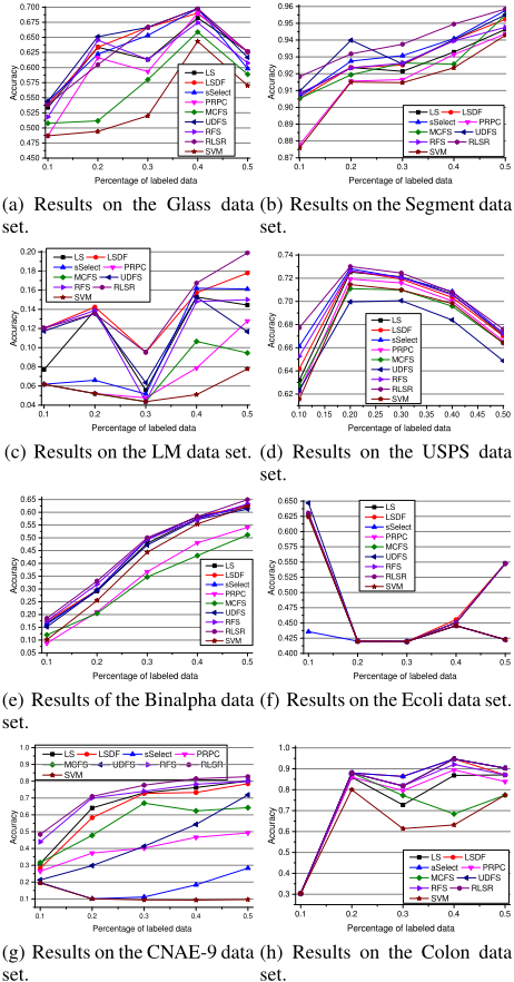
The maximum accuracies of eight feature selection methods versus the percentage of labeled records are shown in Figure 1. In general, the more labeled data we have, the better accuracy we can achieve. This indicates that we are able to select features with higher quality if more labeled data is available. Overall, the proposed method RLSR outperformed other methods on most cases. For example, on the CANE9 data set, RLSR has 4% average improvement compared to the second best approach RFS. 3% average improvement was
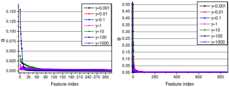
- (a) Results of the Binalpha data set. (b) Results on the CNAE-9 data set.
Figure 2: θ versus different γ.
achieved by the proposed method RLSR on the LM data set, compared to the second best approach LSDF. We also notice that RLSR outperformed RFS on almost all cases, which indicates that RLSR can improve RFS with the unlabeled data. This verifies the effectiveness of the semi-supervised feature selection method.
4.3 Parameter Sensitivity Study
We show the effect of γ on the performance of RLSR in this section. The relationship between γ and θ is shown in Figure 2. For brevity, we only show the results on two data sets (i.e., the Binalpha and CNAE-9 data sets). As γ increased from 0.001 to 1000, the high weights in θ occurred on fewer features. With the increase of γ, θ will contain more values which are close to zero. In real applications, we hope that θ only contains a few features with high weights. Therefore, we can use γ to control the distribution of θ.
In RLSR, γ is used to control the row sparsity of W, and its value seriously influences the final performance. Varying the value of γ, the average clustering accuracies on two data sets are shown in Figure 3. This indicates that RLSR did not change much with the change of γ. In real life applications, we can perform hierarchy grid search to get better result.
4.4 Convergence Study
We have proposed Algorithm 1 to iteratively solve problem (12), and proved its convergence in the previous section. Now we experimentally show the speed of its convergence. The convergence curves of the objective value on two data sets are shown in Figure 4. We can see that, Algorithm 1 converged very fast, which ensures the speed of the whole proposed approach.
5 Conclusions
In this paper, we have proposed a novel semi-supervised feature selection approach named RLSR. The new method extends the least square regression by rescaling the regression coefficients in the least square regression with a set of scale factors, which are used to rank the features. We have proved that the new model can learn both global and sparse solution. Moreover, the optimal solution of scale factor provides a theoretical explanation for why we can use {∥∥w1∥∥2 , ..., ∥∥wd∥∥2 } to rank the features. We have proposed a simple yet effective algorithm with proved convergence to solve the new model. Empirical studies have been performed on eight data sets,
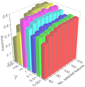
- (a) Results of the Binalpha data set.
- (a) Results of the Binalpha data set. (b) Results on the CNAE-9 data set.
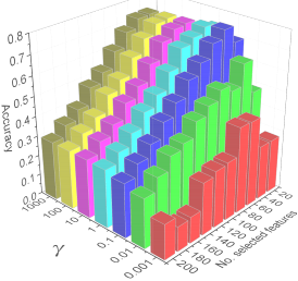
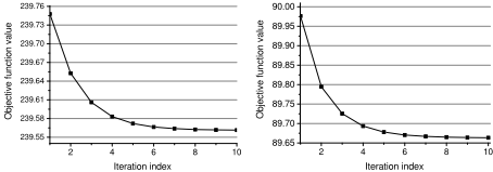
Figure 4: The objective value versus the number of iterations.
to demonstrate the superior performance of our method over seven commonly-used feature selection methods. In the future work, we will improve this method to handle large scale data.
Acknowledgements
This research was supported by NSFC under Grant no.61305059, 61473194 and U1636202.
@inproceedings{ijcai2017p211,
  title     = {Semi-supervised Feature Selection via Rescaled Linear Regression},
  author    = {Chen, Xiaojun and Yuan, Guowen and Nie, Feiping and Huang, Joshua Zhexue},
  booktitle = {Proceedings of the Twenty-Sixth International Joint Conference on
               Artificial Intelligence, {IJCAI-17}},
  publisher = {International Joint Conferences on Artificial Intelligence Organization},
  editor    = {Carles Sierra},
  pages     = {1525--1531},
  year      = {2017},
  month     = {8},
  note      = {Main track},
  doi       = {10.24963/ijcai.2017/211},
  url       = {https://doi.org/10.24963/ijcai.2017/211},
}
TY - CPAPER TI - Semi-supervised Feature Selection via Rescaled Linear Regression AU - Chen, Xiaojun AU - Yuan, Guowen AU - Nie, Feiping AU - Huang, Joshua Zhexue T2 - Proceedings of the Twenty-Sixth International Joint Conference on Artificial Intelligence, IJCAI-17 PB - International Joint Conferences on Artificial Intelligence Organization PY - 2017 SP - 1525 EP - 1531 DO - 10.24963/ijcai.2017/211 UR - https://doi.org/10.24963/ijcai.2017/211 ER -Copied
Machine-readable versions of this paper, for tools and AI agents:





