
Fleet Design Optimisation from Historical Data Using Constraint Programming and Large Neighbourhood Search
Proceedings of the Twenty-Fifth International Joint Conference on Artificial Intelligence. Pages 4185-4188.
© 2016 International Joint Conferences on Artificial Intelligence
Abstract
We present an original approach to compute efficient mid-term fleet configurations at the request of a Queensland-based long-haul trucking carrier. Our approach considers one year's worth of demand data, and employs a constraint programming (CP) model and an adaptive large neighbourhood search (LNS) scheme to solve the underlying multi-day multi-commodity split delivery capacitated vehicle routing problem. This paper is an adaptation of the Best Application Paper at CP'15, published in the Constraints journal with the same title.
- [Archetti and Speranza, 2008] Claudia Archetti and Maria- Grazia Speranza. The split delivery vehicle routing prob- lem: A survey. In Bruce Golden, S. Raghavan, and Ed- ward Wasil, editors, The Vehicle Routing Problem: Lat- est Advances and New Challenges, volume 43 of Opera- tions Research/Computer Science Interfaces, pages 103- 122. Springer US, 2008.
- [Belfiore and Yoshizaki, 2013] Patrícia Belfiore and Hugo T.Y. Yoshizaki. Heuristic methods for the fleet size and mix vehicle routing problem with time windows and split deliveries. Computers & Industrial Engineering, 64(2):589-601, 2013.
- [Bräysy et al., 2008] Olli Bräysy, Wout Dullaert, Geir Hasle, David Mester, and Michel Gendreau. An effective mul- tirestart deterministic annealing metaheuristic for the fleet size and mix vehicle-routing problem with time windows. Transportation Science, 42(3):371-386, 2008.
- [Crainic, 2003] Teodor Gabriel Crainic. Long-haul freight transportation. In Randolph W. Hall, editor, Handbook of Transportation Science, volume 56 of International Series in Operations Research & Management Science, pages 451-516. Springer US, 2003.
- [Dantzig and Ramser, 1959] George B Dantzig and John H Ramser. The truck dispatching problem. Management sci- ence, 6(1):80-91, 1959.
- [Dell'Amico et al., 2007] Mauro Dell'Amico, Michele Monaci, Corrado Pagani, and Daniele Vigo. Heuristic approaches for the fleet size and mix vehicle routing problem with time windows. Transportation Science, 41(4):516-526, 2007.
- [Di Gaspero and Urli, 2014] Luca Di Gaspero and Tommaso Urli. A cp/lns approach for multi-day homecare schedul- ing problems. In Hybrid Metaheuristics, pages 1-15. Springer, 2014.
- [Di Gaspero et al., 2015] Luca Di Gaspero, Andrea Rendl, and Tommaso Urli. Balancing bike sharing systems with constraint programming. Constraints, pages 1-31, 2015.
- [Dror and Trudeau, 1989] Moshe Dror and Pierre Trudeau. Savings by split delivery routing. Transportation Science, 23(2):141-145, 1989.
- [Dror and Trudeau, 1990] Moshe Dror and Pierre Trudeau. Split delivery routing. Naval Research Logistics (NRL), 37(3):383-402, 1990.
- [Kilby and Shaw, 2006] Philip Kilby and Paul Shaw. Vehi- cle routing. Handbook of constraint programming, pages 799-834, 2006.
- [Kilby and Urli, 2015] Philip Kilby and Tommaso Urli. Fleet design optimisation from historical data using constraint programming and large neighbourhood search. Con- straints, pages 1-20, 2015.
- [Kytöjoki et al., 2007] Jari Kytöjoki, Teemu Nuortio, Olli Bräysy, and Michel Gendreau. An efficient variable neighborhood search heuristic for very large scale vehi- cle routing problems. Computers & Operations Research, 34(9):2743-2757, 2007.
- [Pisinger and Ropke, 2010] David Pisinger and Stefan Ropke. Large neighborhood search. In Handbook of Metaheuristics, pages 399-419. Springer, 2010.
- [Ropke and Pisinger, 2006] Stefan Ropke and David Pisinger. An adaptive large neighborhood search heuristic for the pickup and delivery problem with time windows. Transportation science, 40(4):455-472, 2006.
- [Schulte et al., 2015] Christian Schulte, Guido Tack, and Mikael Z. Lagerkvist. Modeling and Programming with Gecode. Schulte, Christian and Tack, Guido and Lagerkvist, Mikael Z., 2015.
- [Shaw, 1998] Paul Shaw. Using constraint programming and local search methods to solve vehicle routing problems.
- In Michael J. Maher and Jean-Francois Puget, editors, CP'98: the 4th International Conference on Principles and Practice of Constraint Programming, 1998, Proceed- ings of, volume 1520 of Lecture Notes in Computer Sci- ence, pages 417-431. Springer, 1998.
- [Toth and Vigo, 2002] Paolo Toth and Daniele Vigo. The Ve- hicle Routing Problem. Society for Industrial and Applied Mathematics, 2002.
- [Vidal et al., 2014] Thibaut Vidal, Teodor Gabriel Crainic, Michel Gendreau, and Christian Prins. A unified solution framework for multi-attribute vehicle routing problems. European Journal of Operational Research, 234(3):658- 673, 2014.
References were extracted automatically from the PDF and may contain errors.
Full text extracted automatically from the PDF; figures, tables and equations may differ. The PDF is the version of record.
1 Introduction
Long-haul transportation is a fundamental component of every country's economy, supporting both the movement of raw materials between production facilities and the delivery of final products to their ultimate destinations [Crainic, 2003]. Transportation also represents a significant fraction of the final price of goods, and making an efficient use of the available transportation infrastructure and resources is essential to reduce costs and remain profitable in the open market.
At the core of most logistics applications lies the vehicle routing problem (VRP) [Dantzig and Ramser, 1959] (see [Toth and Vigo, 2002] for a survey), which consists in dispatching a fleet of vehicles to satisfy the demand of a set of customers. Because of its industrial relevance, the VRP has been often extended to integrate real-world constraints, e.g., compartments, time windows, etc., originating a class of problems denominated "rich" vehicle routing problems. One of such variants, the split delivery vehicle routing problem (SDVRP), is a generalisation of the VRP in which the demand of one customer can be cumulatively satisfied by multiple vehicles. It has been shown [Dror and Trudeau, 1989] that SDVRP can yield considerable savings with respect to the classic VRP, in addition to being, in some circumstances, the only available option. However, while the VRP is itself NP-complete, the SDVRP, as many other rich VRP variants, is NP-hard [Dror and Trudeau, 1990]. Both VRP and SDVRP assume a given fleet of vehicles. The problem of how to design such a fleet is called the fleet size and mix vehicle routing problem (FSMVRP), and is often studied as a generalisation of the VRP where the fleet is not specified in advance, but has to be constructed by the solver from a collection of available vehicle types. Such formulation is appropriate for applications in which the same routing plan is repeated every day, e.g., mail delivery and collection, however it is insufficient to address fleet design for carriers dealing with a variable daily demand. To the best of our knowledge the problem of designing the best fleet for a long planning horizon has not been addressed yet for the general case.
1 This paper is an adaptation of the Best Application Paper at CP'15, published in the Constraints journal [Kilby and Urli, 2015].
In this paper, we take an optimisation perspective on the design of a robust and efficient fleet to support the customer demand over a mid-term, e.g., few months to one year, planning horizon. Our study is carried out at the request of a longhaul carrier operating in the Queensland area in Australia.
2 Related work
A brief review of the relevant literature follows. In [Crainic, 2003], the author surveys long-haul transportation as a whole, highlighting the decisions at the strategic (long-term) level, tactical (mid-term) level, and operational (short-term) level. An important insight in this regard, is that decisions at each level constrain the decisions at the following level, and inform the decisions at the previous level. Dell'Amico et al. [Dell'Amico et al., 2007] present a heuristic solution to the fleet size and mix for the single-day single-commodity vehicle routing problem with time windows, based on a previous linear programming formulation of the same problem. Vidal et al. [Vidal et al., 2014] propose a component-based framework to solve a variety real-world VRP variants, including fleet size and mix vehicle routing. Neither approach handles split deliveries or multiple commodities. In [Archetti and Speranza, 2008] a survey of split delivery vehicle routing is provided, along with a classic linear programming formulation and a thorough discussion of complexity aspects and lower bounds. [Belfiore and Yoshizaki, 2013] describe a scatter search approach to solve the fleet mix problem for the daily split delivery vehicle routing problem. [Br¨aysy et al., 2008] introduce a multi-phase local search approach for the FSMVRP, also considering acquisition costs. None of the above works consider fleet mix aspects, or consider them only in single-day and single-commodity scenarios.
With respect to the reviewed literature, our approach introduces the following novelties. First and foremost, we consider the fleet mix problem in a mid-term perspective, i.e., we seek to find a single fleet design to support the demand across a planning horizon spanning months to years. Second, we consider a multi-commodity split delivery vehicle routing problem, which is very common in real-world industrial contexts. Finally, we propose a Pareto-based technique to extract guaranteed representative subsets of days from the historical data, and to make the problem more tractable.
3 The problem
Our client serves a set of customers c 2 C with locations lc 2 L, and faces a daily multi-commodity, split delivery, long-haul vehicle routing problem, to be addressed using a heterogeneous fleet of trucks. On a daily basis, each customer c 2 C may issue an order for a quantity qc↪k 2 Z⇤ of some commodity k 2 K. We will use the sets C and L interchangeably. The available vehicle types t 2 T to carry out the deliveries differ in i) their total capacity, denoted by bt, ii) the commodities that can be transported, specified through a Boolean compatibility relation compt↪k, and iii) the operation cost per kilometre, denoted by wt. Table 1 reports the described parameters for the considered vehicle types. Following our client's requirements, goods must be picked up from a central depot, denoted by dep, where the vehicles must return at the end of the day. We are given the distance in kilometres, distli↪lj , between each pair of locations li↪ lj 2 L[¶ldep♦. Our client handles the delivery of refrigerated (or chilled) and non-refrigerated (or ambient) products, but only some of the vehicle types are refrigerated. Ambient goods can be transported in all vehicles. The above problem
| # | Model | wt | bt | Refrigerated |
|---|---|---|---|---|
| 0 | B-Double | 2.59 | 34 | no |
| 1 | A-Double | 2.67 | 40 | no |
| 2 | B-Triple | 2.86 | 48 | no |
| 3 | B-Double Reefer | 2.99 | 34 | yes |
| 4 | A-Double Reefer | 3.04 | 40 | yes |
can be seen in two perspectives. At the operational (day to day) level, we want to load and route a given fleet of vehicles so that the daily demand of all the customers is met, the vehicle capacities and compatibilities are respected, and the total operation cost is minimised. At the tactical level, given an unlimited availability of each type of vehicle, we want to design a fleet with enough capacity to support the operations over the mid-term based on one year of historic demand data.
4 Proposed approach
Following the principle, expressed in [Crainic, 2003], that decisions at the tactical level must be informed by the decisions at the operational level, we propose to solve the fleet mix problem by lifting the daily loading and routing problem to a multi-day perspective, and by relaxing the fixed fleet constraint 2 . This allows our method to find the most suitable fleet design across the multi-day horizon, instead of producing a different fleet for each day.
2 By "relaxing" we mean that the fleet is not given a priori, but chosen by the solver and then used for the whole horizon.
The multi-day extension of the problem over a horizon D = ¶0↪ ▷ ▷ ▷ ↪ D - 1♦ of D days, is obtained by augmenting the demand qc↪k with an additional index d indicating which day it belongs to (qd↪c↪k). Moreover, we assume a bound V on the maximum number of vehicles in the fleet, and we denote the set of all possible vehicles indices as V = ¶0↪ ▷ ▷ ▷ ↪ V -1♦. Finally, for model compactness, on each day d 2 D we only consider the customers Cd ✓ C for which qd↪c↪k > 0.
4.1 Model
We solve the above problem by means of an adaptive large neighbourhood search (LNS) procedure built on top of a constraint programming (CP) model. Our model is inspired by the multi-day vehicle routing approach described in [Di Gaspero and Urli, 2014], but follows a step-based formulation in which each route is encoded as a fixed-length sequence of "visits", rather than the classic vehicle routing formulation in which, for each customer, a "successor" variable points to the next customer. The step-based formulation, similar to the one proposed in [Di Gaspero et al., 2015], is extremely suitable for handling split delivery problems, unlike successor-based formulations where, in order to allow multiple visits to the same customer, one has to use n - 1 "virtual" customers, where n is the maximum number of visits. Moreover, unlike both [Di Gaspero and Urli, 2014; Di Gaspero et al., 2015], our model can handle multiple commodities and a flexible (albeit bounded) fleet. For space reasons, we are unable to provide a complete discussion of the constraints (see [Kilby and Urli, 2015] for the full model), however these can be derived from the description of the problem and of the modelling variables.
The variables in our model can be classified in two sets. The first set represents horizon-wide decisions, describing the overall composition of the fleet. For each vehicle v 2 V a variable v typev with domain ¶0↪ ▷ ▷ ▷ ↪ ♣T♣♦ represents the type of the vehicle (the vehicle type with index ♣T♣ being assigned to all unused vehicles). A Boolean variable usedv models whether a given vehicle is part of the fleet or not. Finally, an integer variable n veh, with domain ¶1↪ ▷ ▷ ▷ ↪ V ♦, represents the number of vehicles which are part of the fleet. The second set of variables represent daily decisions. For each day d 2 D, and each vehicle v 2 V a Boolean variable, used ond↪v, models whether vehicle v 2 V is used on day d. Similarly, for each day d 2 D, the variable n veh ond models the number of vehicles used on day d. Note that the type and the general availability of each vehicle is decided at the horizon level, but not all the vehicles need to be used every day. Routes are constructed as sequences of steps (visits to customers). We denote the set of steps in a day d 2 D as Sd = ¶0↪ ▷ ▷ ▷ ↪ ♣Cd♣ + 1♦. The number of daily steps is the number of customers ♣Cd♣ with non-zero demand on day d plus two steps for the initial and final visits to the depot. The arbitrary bound on the route length is motivated by the fact that in long-haul contexts it is very unlikely that the same customer be visited twice by the same vehicle. For each day d 2 D, each vehicle v 2 V, and each step s 2 Sd, an integer variable visd↪v↪s, with domain ¶0↪ ▷ ▷ ▷ ↪ ♣Cd♣♦, represents the s-th visit of vehicle v on day d. The values 0 (or null) and 1 (or dep) in the domain of vis are reserved, respectively, for unused steps and for visits to the depot. Note that null visits can only appear at the end of a route, and allow for routes shorter than ♣Sd♣. Regarding vehicle loading, for each day d 2 D, for each vehicle v 2 V, for each step s 2 Sd, and for each commodity k 2 K, an integer variable loadd↪v↪k↪s represents the amount of k left on v after step s is performed on day d. In order to define the cost measure, we also need a few auxiliary variables. For each day d 2 D, each vehicle v 2 V, and each step s 2 Sd, the total distance travelled up to step s by vehicle v on day d is represented with an integer variable tot distd↪v↪s. Similarly, for each d 2 D, and each vehicle v 2 V, the daily operation cost of vehicle v is modelled with a floating point variable tot costd↪v with a domain going from zero to the maximum vehicle distance multiplied by maxt2Twt. Finally, a tot cost variable aggregates the daily vehicles costs through a sum constraint, providing the overall cost measure for a given solution s. During an optimisation run, the value of tot cost is dynamically upperbounded by the cost of the best solution ˆ s found so far, so as to only produce improving solutions.
4.2 Search
Large neighbourhood search (LNS) [Shaw, 1998; Pisinger and Ropke, 2010] is a local search meta-heuristic based on the observation that exploring a large neighbourhood, i.e., modifying a large portion of an existing one, tends to yield solutions of higher quality wrt. exploring a small neighbourhood. To make this exploration efficient, LNS has often been coupled with filtering techniques, such as constraint propagation, that contain the size of the neighbourhood by culling lowquality or unfeasible solutions. In our approach, we use the presented CP model as a source of propagation, and we use a branch & bound tree-search strategy to explore the neighbourhood of the incumbent solution. Similar approaches have been applied to tackle several vehicle routing problem variants [Kilby and Shaw, 2006; Ropke and Pisinger, 2006; Kyt¨ojoki et al., 2007].
We define two different search strategies, consisting of different variable and value selection heuristics. The first is used to find the initial solution for LNS. The second is used during the re-optimisation in the repair step of LNS.
Strategy 1. First, the total number of vehicles and their types are chosen, prioritising small fleets and large vehicles. After the fleet has been chosen, we proceed day by day. First we choose how many and which vehicles are dispatched (the fewer the better). Then we handle the loading and routing aspects vehicle by vehicle, trying to maximise their utility. To do this, we load as much as possible at the depot and we unload as much as possible at the customers. After a vehicle returns to the depot, we move on to the next, until all the demand is satisfied.
Strategy 2. This strategy differs from the previous only with respect to the value selection heuristic, which chooses values uniformly at random within the variables domains, except for the number of vehicles and the initial loads which follow the same principles of Strategy 1.
These strategies, combined with the constraints on the capacity of the fleet, allows us to detect unfeasible fleets early, even in multi-day scenarios. Once the first solution is generated using Strategy 1, the search enters a refinement loop which alternates two steps. First, a destroy (or relax) procedure sets a subset of the decision variables to their original domains, and propagates the model's constraints until a fix point is reached. After this step we are left with a smaller problem, which is much easier to optimise. Second, a repair procedure, consisting of a branch & bound tree-search based on Strategy 2 re-optimises the newly freed variables yielding a new solution. Since the cost of the next solution is dynamically bounded, only improving solutions are generated. Our destroy phase employs two different relaxation schemes, selected with coin-toss probability and parametrised with a parameter δ, the destruction rate, representing the intensity of the relaxation
Relax δ days. all the decision variables (of all vehicles) concerning δ days chosen uniformly at random are relaxed,
Relax δ vehicles. all the decision variables (across all days) related to δ vehicles, chosen uniformly at random between the ones currently used in the solution plus the first unused vehicle, are relaxed.
The parameter δ represents the adaptive part of our LNS procedure. It is initialised to 1, and increased by one every time itermax iterations (a parameter of the solver) have been spent on a value of δ without improvement. Once an improving solution is found, δ is re-set to 1. If no improving solution are found, but δ cannot be further increased, the search is restarted from a new initial solution. In our setup, each repair step is given a time budget of nfree · tvar milliseconds, where nfree is the number of variables relaxed by the destroy step, and tvar is a parameter of the solver.
4.3 Pre-processing
Solving multi-day problems for long planning horizons, e.g., one year, is computationally hard. The particular nature of our problem, allows us to do better. Using a Pareto dominance-based approach, we identify representative subsets of the historical data, and use those in place of the whole horizon. To accomplish this, we represent each day d in the horizon with the total amount of ambient and chilled demand, i.e., (qd↪amb↪ qd↪chi), and consider these as objectives to be maximised. The idea behind our approach is that, if the demand on a day p dominates the demand on a day q, then the optimal fleet for p is also guaranteed to be able to serve q. By extending this reasoning to the multi-day perspective, we can state that a fleet which can solve the multi-day problem based on the Pareto front of the days is also guaranteed to be able to solve all the other days.
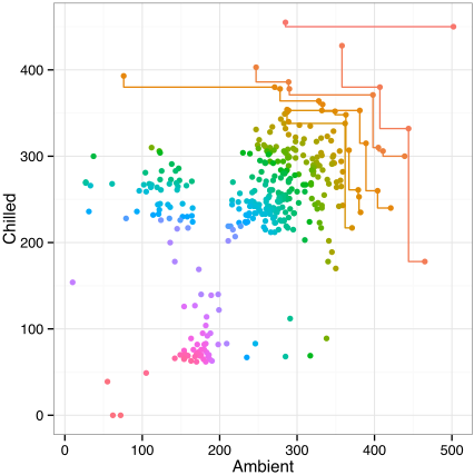
We computed the Pareto front based on 364 days of historical order data. The front is composed by only two days, which greatly dominate the other ones. We identified the optimal fleet for such front (we call this the conservative fleet), and then we tested it on each day of the horizon. These experiments revealed that, while the identified fleet guarantees a coverage of 100% of the days, almost half of the vehicles were unused, on average, in a typical day. For this reason we decided to adopt a layered Pareto approach, in which multiple Pareto fronts, with decreasing degrees of coverage (but increasing levels of efficiency), are generated. The algorithm, discussed extensively in [Kilby and Urli, 2015], proceeds by identifying the Pareto front, removing the days belonging to it from the horizon, and identifying the next one, until there are no more days left. In particular, starting from the 364 days, it identifies 46 fronts with decreasing instance coverage. In Figure 1, we show the annual distribution of chilled and ambient goods demand, highlighting the first six fronts. These contain less than 10 days each, and dominate 100% (front 0, upper right) to 90% (front 5, lower left) of the days.
5 Experimental analysis
We report the major findings from the experimental evaluation. The full discussion of the results, including a comparison between branch & bound, LNS, and a MIP formulation of the problem, can be found in [Kilby and Urli, 2015].
We implemented our CP model and LNS scheme in GECODE 4.4.0 [Schulte et al., 2015] and then carried out an experimental analysis to identify the best fleet for each of the first six fronts. The problem instances considered in our experimental analysis represent the same 364 days used to identify the Pareto fronts. The instances have a median of 19 customers per day, with the total demand evenly distributed between ambient and chilled goods. The tuning of the LNS parameters is described in [Kilby and Urli, 2015]; the final values identified by the tuning procedure are itermax = 20 and tvar = 1 millisecond.
We solved the multi-day instances obtained aggregating the days in the Pareto fronts identified in the pre-processing phase. In these experiments we used a maximum number of vehicles of V = 25. All the experiments were run on a cluster of 3▷1 GHz AMD Opteron nodes with 64 GB of RAM
each and allotted 1 hour of time. The identified fleets differ in size (see Table 2) but share the same composition: the only used vehicles are the largest non-refrigerated and refrigerated trucks, respectively B-Triples and A-Double Reefers.
| F | V | Costd | Coverage | Cost% | Usage |
|---|---|---|---|---|---|
| 0 | 22 | 51.71k | 100.00% | 8.60% | 52.92% |
| 1 | 19 | 52.24k | 99.73% | 9.88% | 62.37% |
| 2 | 18 | 51.71k | 98.90% | 8.69% | 64.74% |
| 3 | 17 | 51.79k | 97.80% | 8.78% | 68.55% |
| 4 | 17 | 52.22k | 97.25% | 9.86% | 69.70% |
| 5 | 17 | 52.66k | 96.98% | 10.92% | 70.50% |
We then validated each fleet independently on all the daily instances by running the solver for 15 minutes. The results of our analysis are summarised in Table 2 reporting, for every identified fleet,i) the number of vehicles (V), ii) the average daily operations cost (Costd), iii) the actual instance coverage, iv) the difference in daily cost between using the Paretobased fleet vs. the ideal fleet for each day (Cost%), and v) the average utilisation of vehicles on each day (Usage). Note that the cost of the ideal fleet for each day is a measure of the absolute best we can do, and represents an goal rather than a viable alternative. From our results emerges that, by optimising the usage of resources, it is possible to maintain a good instance coverage while reducing the fleet size. A metric that provides insight on the quality of a fleet is the average daily utilisation of vehicles. Good fleets tend to have a high utilisation rate. For instance, with an average operation cost of about 9% above the the ideal fleet, the fleet based on the 2nd Pareto front achieves an instance coverage of almost 99% using 4 vehicles less than the conservative fleet.
6 Conclusions
We proposed i) a constraint programming model for the multi-day, multi-commodity, fleet mix and routing problem, ii) a large neighbourhood scheme to produce daily plans and efficient fleet designs using the proposed model as a propagation engine, and iii) a pre-processing phase that allows us to use subsets of instances to predict the best fleet based on the historical demand data. The main novelty of our approach lies in how we use a solver for short-term operational decisions (routing and loading) to inform the mid-term tactical decisions (fleet design), and in our pre-processing technique.
Our approach has also a number of limitations. First, our pre-processing phase relies on the fact that the instance coverage of a fleet can be easily calculated by looking at the total demand. This is not necessarily the case if side constraints, e.g., time windows, are added to the model. While it is relatively easy to add constraints to a CP model, the lack of an effective pre-processing phase can limit substantially our ability to to handle large horizons. Second, our approach does not take into account the costs of modifying the fleet and hiring on-demand vehicles. These aspects must be considered to provide a holistic view to the client. These aspects are presently under investigation.
@inproceedings{ijcai2016p627,
  title     = {Fleet Design Optimisation from Historical Data Using Constraint Programming and Large Neighbourhood Search},
  author    = {Kilby, Philip and Urli, Tommaso},
  booktitle = {Proceedings of the Twenty-Fifth International Joint Conference on
               Artificial Intelligence, {IJCAI-16}},
  publisher = {AAAI Press / International Joint Conferences on Artificial Intelligence},
  editor    = {Subbarao Kambhampati},
  pages     = {4185--4188},
  year      = {2016},
  month     = {7},
  url       = {https://ijcai.org/proceedings/2016/627},
}
TY - CPAPER TI - Fleet Design Optimisation from Historical Data Using Constraint Programming and Large Neighbourhood Search AU - Kilby, Philip AU - Urli, Tommaso T2 - Proceedings of the Twenty-Fifth International Joint Conference on Artificial Intelligence, IJCAI-16 PB - AAAI Press / International Joint Conferences on Artificial Intelligence PY - 2016 SP - 4185 EP - 4188 UR - https://ijcai.org/proceedings/2016/627 ER -Copied
Machine-readable versions of this paper, for tools and AI agents:





