
Incorporating Prototype Theory in Convolutional Neural Networks
Proceedings of the Twenty-Fifth International Joint Conference on Artificial Intelligence. Pages 3446-3452.
© 2016 International Joint Conferences on Artificial Intelligence
Abstract
Deep artificial neural networks have made remarkable progress in different tasks in the field of computer vision. However, the empirical analysis of these models and investigation of their failure cases has received attention recently. In this work, we show that deep learning models cannot generalize to atypical images that are substantially different from training images. This is in contrast to the superior generalization ability of the visual system in the human brain. We focus on Convolutional Neural Networks (CNN) as the state-of-the-art models in object recognition and classification; investigate this problem in more detail, and hypothesize that training CNN models suffer from unstructured loss minimization. We propose computational models to improve the generalization capacity of CNNs by considering how typical a training image looks like. By conducting an extensive set of experiments we show that involving a typicality measure can improve the classification results on a new set of images by a large margin. More importantly, this significant improvement is achieved without fine-tuning the CNN model on the target image set.
- [Agrawal et al., 2014] Pulkit Agrawal, Dustin Stansbury, Ji- tendra Malik, and Jack L Gallant. Pixels to voxels: Model- ing visual representation in the human brain. arXiv preprint arXiv:1407.5104, 2014.
- [Ashby and Alfonso-Reese, 1995] F Gregory Ashby and Le- ola A Alfonso-Reese. Categorization as probability den- sity estimation. Journal of mathematical psychology, 39(2):216-233, 1995.
- [Bengio et al., 2009] Yoshua Bengio, Jérôme Louradour, Ro- nan Collobert, and Jason Weston. Curriculum learning. In Proceedings of the 26th annual international conference on machine learning, pages 41-48. ACM, 2009.
- [Blum and Langley, 1997] Avrim L Blum and Pat Langley. Selection of relevant features and examples in machine learning. Artificial intelligence, 97(1):245-271, 1997.
- [Bo et al., 2010] Liefeng Bo, Xiaofeng Ren, and Dieter Fox. Kernel descriptors for visual recognition. In NIPS, 2010.
- [Cadieu et al., 2014] Charles F Cadieu, Ha Hong, Daniel LK Yamins, Nicolas Pinto, Diego Ardila, Ethan A Solomon, Najib J Majaj, and James J DiCarlo. Deep neural networks rival the representation of primate it cortex for core visual object recognition. PLoS computational biology, 2014.
- [Crammer and Singer, 2002] Koby Crammer and Yoram Singer. On the algorithmic implementation of multiclass kernel-based vector machines. JMLR, 2002.
- [Deng et al., 2009] Jia Deng, Wei Dong, Richard Socher, Li- Jia Li, Kai Li, and Li Fei-Fei. Imagenet: A large-scale hierarchical image database. In Computer Vision and Pat- tern Recognition, 2009. CVPR 2009. IEEE Conference on, pages 248-255. IEEE, 2009.
- [Feldman, 2000] Jacob Feldman. Bias toward regular form in mental shape spaces. Journal of Experimental Psychology: Human Perception and Performance, 2000.
- [Fukushima, 1980] Kunihiko Fukushima. Neocognitron: A self-organizing neural network model for a mechanism of pattern recognition unaffected by shift in position. Biolog- ical cybernetics, 36(4):193-202, 1980.
- [Fukushima, 2013] Kunihiko Fukushima. Artificial vision by multi-layered neural networks: Neocognitron and its ad- vances. Neural Networks, 37:103-119, 2013.
- [Ghodrati et al., 2014] Masoud Ghodrati, Amirhossein Farzmahdi, Karim Rajaei, Reza Ebrahimpour, and Seyed- Mahdi Khaligh-Razavi. Feedforward object-vision models only tolerate small image variations compared to human. Frontiers in computational neuroscience, 2014.
- Goodman et al., ] Noah D Goodman, Joshua B Tenenbaum, Jacob Feldman, and Thomas L Griffiths. A rational analy- sis of rule-based concept learning. Cognitive Science. [He et al., 2015]
- Kaiming He, Xiangyu Zhang, Shaoqing Ren, and Jian Sun. Delving deep into rectifiers: Surpassing human-level performance on imagenet classification. arXiv preprint arXiv:1502.01852, 2015.
- [Hubel and Wiesel, 1962] David H Hubel and Torsten N Wiesel. Receptive fields, binocular interaction and func- tional architecture in the cat's visual cortex. The Journal of physiology, 160(1):106, 1962.
- [Jia et al., 2014] Yangqing Jia, Evan Shelhamer, Jeff Don- ahue, Sergey Karayev, Jonathan Long, Ross Girshick, Ser- gio Guadarrama, and Trevor Darrell. Caffe: Convolutional architecture for fast feature embedding. arXiv preprint arXiv:1408.5093, 2014.
- [Khaligh-Razavi and Kriegeskorte, 2014] Seyed-Mahdi Khaligh-Razavi and Nikolaus Kriegeskorte. Deep super- vised, but not unsupervised, models may explain it cortical representation. 2014.
- [Khosla et al., 2015] Aditya Khosla, Akhil Raju S., Antonio Torralba, and Aude Oliva. Understanding and predicting image memorability at a large scale. 2015.
- [Krizhevsky et al., 2012] Alex Krizhevsky, Ilya Sutskever, and Geoffrey E Hinton. Imagenet classification with deep convolutional neural networks. In Advances in neural in- formation processing systems, pages 1097-1105, 2012.
- [Lake et al., 2015] Brenden M Lake, Wojciech Zaremba, Rob Fergus, and Todd M Gureckis. Deep neural networks pre- dict category typicality ratings for images. 2015.
- [LeCun et al., 1989] Yann LeCun, Bernhard Boser, John S Denker, Donnie Henderson, Richard E Howard, Wayne Hubbard, and Lawrence D Jackel. Backpropagation ap- plied to handwritten zip code recognition. Neural compu- tation, 1(4):541-551, 1989.
- [LeCun et al., 1998] Yann LeCun, Léon Bottou, Yoshua Ben- gio, and Patrick Haffner. Gradient-based learning ap- plied to document recognition. Proceedings of the IEEE, 86(11):2278-2324, 1998.
- [LeCun et al., 2015] Yann LeCun, Yoshua Bengio, and Geof- frey Hinton. Deep learning. Nature, 2015.
- [Minda and Smith, 2001] John Paul Minda and J David Smith. Prototypes in category learning: the effects of cat- egory size, category structure, and stimulus complexity. Journal of Experimental Psychology: Learning, Memory, and Cognition, 27(3):775, 2001.
- [Murphy, 2002] G. L. Murphy. The Big Book of Concepts (Bradford Books). The MIT Press, March 2002.
- [Nguyen et al., 2015] Anh Nguyen, Jason Yosinski, and Jeff Clune. Deep neural networks are easily fooled: High con- fidence predictions for unrecognizable images. 2015.
- [Nosofsky, 1984] Robert M Nosofsky. Choice, similarity, and the context theory of classification. J. of Experimental Psy- chology: Learning, memory, and cognition, 1984.
- [Pinto et al., 2008] N. Pinto, D. Cox, and J. J DiCarlo. Why is real-world visual object recognition hard? 2008.
- [Rips, 1975] L. J. Rips. Inductive judgments about natural categories. Journal of verbal learning and verbal behavior, 14:665-681, 1975.
- [Rosch, 1978] E. Rosch. Principles of categorization. In E. Rosch and B. Lloyd, editors, Cognition and categoriza- tion. Lawrence Erlbaum, 1978.
- [Saleh et al., 2013] Babak Saleh, Ali Farhadi, and Ahmed El- gammal. Object-centric anomaly detection by attribute- based reasoning. In Conference on Computer Vision and Pattern Recognition (CVPR). IEEE, 2013.
- [Sermanet et al., 2013] Pierre Sermanet, David Eigen, Xiang Zhang, Michaël Mathieu, Rob Fergus, and Yann LeCun. Overfeat: Integrated recognition, localization and detection using convolutional networks. In ICLR, 2013.
- [Sharif Razavian et al., 2015] Ali Sharif Razavian, Josephine Sullivan, Atsuto Maki, and Stefan Carlsson. A baseline for visual instance retrieval with deep convolutional networks. In ICLR, 2015.
- [Simonyan and Zisserman, 2015] Karen Simonyan and An- drew Zisserman. Very deep convolutional networks for large-scale image recognition. 2015.
- [Sloman, 1993] S.A. Sloman. Feature-based induction. Cog- nitive Psychology, 25:231-280, 1993.
- [Szegedy et al., 2013] Christian Szegedy, Wojciech Zaremba, Ilya Sutskever, Joan Bruna, Dumitru Erhan, Ian Goodfellow, and Rob Fergus. Intriguing properties of neural networks. arXiv preprint arXiv:1312.6199, 2013.
- [Torralba and Efros, 2011] Antonio Torralba and Alexei Efros. Unbiased look at dataset bias. In CVPR, 2011.
- [Vinyals et al., 2014] Oriol Vinyals, Alexander Toshev, Samy Bengio, and Dumitru Erhan. Show and tell: A neural image caption generator. arXiv:1411.4555, 2014.
- [Yamins et al., 2014] Daniel LK Yamins, Ha Hong, Charles F Cadieu, Ethan A Solomon, Darren Seibert, and James J Di- Carlo. Performance-optimized hierarchical models predict neural responses in higher visual cortex. Proceedings of the National Academy of Sciences, 2014.
- [Zhu et al., 2015] Xiangxin Zhu, Carl Vondrick, Charless C Fowlkes, and Deva Ramanan. Do we need more training data? IJCV, 2015.
References were extracted automatically from the PDF and may contain errors.
Full text extracted automatically from the PDF; figures, tables and equations may differ. The PDF is the version of record.
1 Introduction
Convolutional Neural Networks (CNN) have made remarkable progress in a variety of computer vision tasks. To just name few of the recent advances, CNN-based models greatly improved object classification and detection [Simonyan and Zisserman, 2015], image retrieval and scene classification [Sharif Razavian et al., 2015], and image captioning [Vinyals et al., 2014].
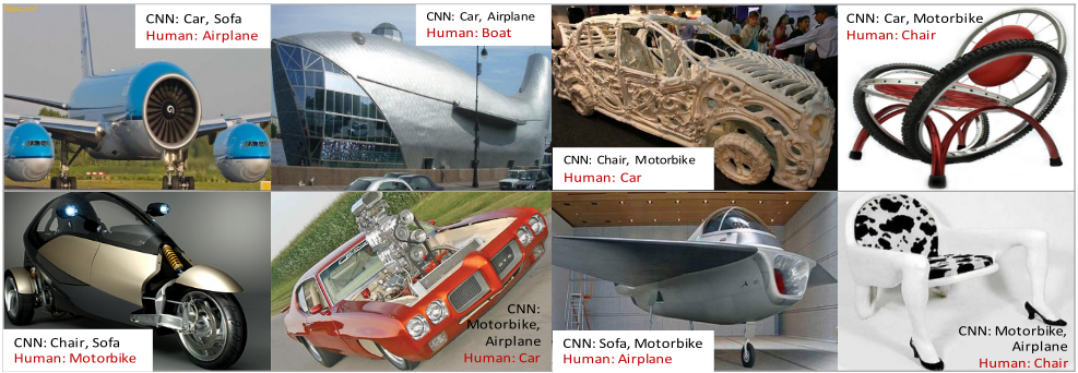
Despite the superior performance on large-scale visual object classification, convolution neural networks cannot emulate the generalization power of the human visual system in real-world object categorization [Ghodrati et al., 2014; Pinto et al., 2008], especially when it comes to objects that differ substantially from the training examples. Figure 1 shows examples of these atypical images, which human subjects categorize correctly, but which a CNN model misclassi-
⇤Corresponding author: babaks@cs.rutgers.edu
Jacob Feldman
Center for Cognitive Science Rutgers University New Jersey, USA
fied with a high confidence. We evaluate the performance of CNNs for the purpose of object classification on atypical images. Humans are capable of perceiving atypical objects and reasoning about them, even though they had not seen them before [Saleh et al., 2013]. But our experiments have shown that state-of-the-art CNNs failed drastically to recognize atypical objects. Table 1 shows the results of this experiment, where we took off-the-shelf CNNs and applied them on atypical images. The significant performance drop, when tested on atypical images, is rooted in the limited generalization power of CNN models versus the human visual system.
One might argue that this issue of cross-dataset generalization is implicitly rooted in dataset biases, and not limited to CNN models [Torralba and Efros, 2011]. However, we argue that the huge number of labeled images in the training set of these models (here ImageNet) should alleviate this drawback. By providing a wide range of variation in terms of visual appearances of objects in training images, the effect of biases fades away. We support our argument by testing same networks on a new set of images that are disjoint from the training set of ImageNet [Deng et al., 2009], but look typical. Results of this experiment as it is reported in columns "Test-T" in Table 1 show a much smaller drop in accuracy, compared to the case of testing on atypical images (Test-A). We conclude that dataset bias can affect the performance of CNNs for object categorization, but it is not the main reason behind its poor generalization to new datasets.
Instead, inspired by the way humans learn object categories, we can empower CNN models with the ability to categorize extremely difficult cases of atypical images. Humans begin to form categories and abstractions at an early age[Murphy, 2002]. The mechanisms underlying human category formation are the subject of many competing accounts, including those based on prototypes[Minda and Smith, 2001], exemplars[Nosofsky, 1984], density estimation[Ashby and Alfonso-Reese, 1995], and Bayesian inference[Goodman et al., ]. But all modern models agree that human category representations involve subjective variations in the typicality or probability of objects within categories. In other words, typicality is a graded concept and there is no simple decision boundary between typical vs. atypical examples. A category like bird, would include both highly typical examples such as robins, as well as extremely atypical examples like penguins and ostriches, which while belonging to the category seem like subjectively "atypical" examples. Visual images can also seem atypical, in that they exhibit features that depart in some way from what is typical for the categories to which they belong. Humans learn object categories and form their visual biases by looking at typical samples [Sloman, 1993; Rips, 1975]. But they are able to generalize these visual concepts to a great extent, and recognize atypical/abnormal objects, which show significant visual variations from the training set. They achieve this ability without even observing abnormal images at the learning stage.
| Method | Top-1 error (%) | Top-5 error (%) | ||||
|---|---|---|---|---|---|---|
| Train | Test-T | Test-A | Train | Test-T | Test-A | |
| AlexNet [Krizhevsky et al., 2012] | 38.1 | 49.5 | 74.96 | 15.32 | 24.01 | 47.07 |
| OverFeat [Sermanet et al., 2013] | 35.1 | 45.36 | 75.62 | 14.2 | 22.27 | 46.73 |
| Caffe [Jia et al., 2014] | 39.4 | 51.88 | 77.12 | 16.6 | 24.74 | 46.86 |
| VGG-16 [Simonyan and Zisserman, 2015] | 30.9 | 44.04 | 77.82 | 15.3 | 26.31 | 47.49 |
| VGG-19 [Simonyan and Zisserman, 2015] | 30.5 | 43.72 | 76.35 | 15.2 | 26.85 | 45.99 |
From computer vision and machine learning perspectives, state-of-the-art object classification and detection is based on discriminative models (e.g. SVM, CNN, Boosting) rather than generative ones. Discriminative training focuses more on learning boundaries between object classes, instead of finding common characteristics in each class. Training CNN models is based on minimization of a loss function, defined as the misclassification of training samples. In that sense, CNN implicitly emphasizes on the boundary examples rather than more representative (typical) training examples.
In this work, we hypothesize that not all images are equally important for the purpose of training visual classifiers, and in particular deep convolutional neural networks. Instead, we show that if training images are weighted based on how typical they look, we can learn visual classifiers with a better generalization capacity. Our final CNN model is fine-tuned only with typical images, but outperforms the baseline model (training samples are not weighted) on dataset of atypical images. We also empirically compare a large set of functions that can be used for weighting samples, and conclude that an even-degree polynomial function of typicality ratings is the best strategy to weight training images. We also investigate the effect of loss functions and depth of network by conducting experiments on two datasets of ImageNet and PASCAL. The main contributions of this paper are as following:
- ÷ Evaluating CNN models on datasets of images that are different from training data, and characterizing failure cases as the poor generalization capacity of CNN models. Especially contrasting these failures to the superior performance of humans in categorizing atypical objects.
- ÷ Inspired by theories in psychology and machine learning, we propose three hypotheses to improve the generalization capacity of CNN models. These hypotheses are based on weighting training images depending on how typical they look. Our final strategy uses generative hints from prototype theory (typicality scores) to improve the generalization capacity of discriminatively
trained CNN classifiers.
- ÷ We conduct an extensive set of experiments, to empirically compare different functions of typicality rating for weighting training images.
2 RelatedWork
Space does not allow an encyclopedic review of the prior literature on deep learning, but we refer interested readers to the literature review of [LeCun et al., 2015]. For our research, we focus on convolutional neural networks [Fukushima, 2013; Krizhevsky et al., 2012; LeCun et al., 1998] as the state-ofthe-art deep learning models for the task of object recognition. CNN [LeCun et al., 1989] has its roots in Neocognitron [Fukushima, 1980], which is a hierarchical model based on the classic notion of simple and complex cells in visual neuroscience [Hubel and Wiesel, 1962]. However, CNN has additional hidden layers to model more complex nonlinearities in visual data and its overall architecture is reminiscent of the LGN 7! V1 7! V2 7! V4 7! IT hierarchy in the visual cortex ventral pathway. Additionally it uses an end-toend supervised learning algorithm, called "Backpropagation" to learn weights of layers. Different variations of CNN models have made breakthrough performance improvements in a variety of tasks in the field of computer vision.
Despite an extensive amount of prior works on applications of CNN and proposed variations of it, theoretical understanding of them remains limited. More importantly, even when CNN models achieve human-level performance on visual recognition tasks [He et al., 2015], what will be the difference between computer and human vision? On the one hand, Szegedy et al.[2013] demonstrated that CNN classification can be severely altered by very small changes to images, where it leads to radically different CNN classification of images that are indistinguishable to the human visual system. On the other hand, Nguyen et al.[2015] generated images that are completely unrecognizable by humans, but which a CNN model would classify them with 99.99% confidence. This strategy to fool CNN models, raises questions about the true generalization capabilities of such models, which we investigate it in this paper.
In addition, recent studies in the field of neuroscience and cognition have shown the connection between deep neural networks (mainly CNN) and the visual system in human brain. Yamins et al.[2014] showed there is a correlation (similarity) between the activation of middle layers of CNN and the brain responses in both V4 and inferior temporal (IT), the top two layers of the ventral visual hierarchy. Cadieu et al.[2014] proposed a kernel analysis approach to show that deep neural networks rival the representational performance of IT cortex on visual recognition tasks. Khaligh-Razavi and Kriegeskorte [2014] studied 37 computational model representations and found out the CNN model of [Krizhevsky et al., 2012] came the closest to explaining the brain representation. Interestingly, the amount of correlation between human IT and layers of CNN increases by moving to higher layers (fully-connected layers). They concluded that weighted combination of features of the last fully connected layer can explain IT to a full extent. It has been shown that CNN models predict human brain activity accurately in early and intermediate stages of the visual pathway [Agrawal et al., 2014].
There are some prior works on finding the right features [Blum and Langley, 1997], choosing the appropriate train set and how to order training examples for learning better classifiers [Bengio et al., 2009]. Also, It has been shown that CNN models benefit from training with larger datasets of images. This is because the greatest gain in detection performance will continue to derive from improved representations and learning algorithms that can make efficient use of larger training sets [Zhu et al., 2015]. However, this leaves open the question if training images should be equally weighted during the training or not?
3 Computational Framework
In this section, we first review some through theoretical background and compelling theories about the learning of visual concepts in both fields of psychology and computer vision. We explain the role of atypical examples in training classifiers, and how one can measure the typicality of objects in an image. Then we propose three hypotheses to use these typicality scores for improving the generalization capacity of visual classifiers.
3.1 FrameworkMotivation
Humans learn a visual object class by looking at examples that are more representative for that object category, or what is called typical samples [Sloman, 1993; Rips, 1975]. It has been shown that children who learn a category by looking at more typical samples, later can recognize its members better [Rosch, 1978]. If training examples look more typical, they fall close to each other in an underlying space of visual features. This learning strategy not only helps humans to form a concept, but also allows them to more easily apply the learned concept to novel images. This great ability of human visual system allows them to recognize completely different variations of an object, even to the extent of atypical ones. This suggests that emphasizing on typical examples might be helpful for improving the generalization capacity of classifiers.
However, state-of-the-art object classifiers in computer vision are discriminative models, where they distinguish different objects by learning category boundaries. CNN models as discriminative deep neural networks have multiple layers to learn a hierarchy of visual features and categorize objects by minimizing a loss function, which is based on misclassification errors. In other words, if an image is classified correctly (usually the case for typical images), it has little or no impact on the loss function, hence can be ignored in the training phase. This implies that examples close to the decision boundary, which are likely to be more atypical images, play a substantial role in learning CNN models. This suggests that CNN training emphasizes on more atypical images to learn visual classifiers with a better performance.
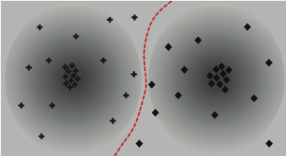
We illustrates the connection between typical, atypical, boundary and misclassified training samples in Figure 2; where examples of two object classes (C) are shown with diamonds and crosses, and the red dotted line is one possible decision boundary. There are two main points to be taken from this illustration:
First, as we discussed in Section 1 typicality is a graded concept, which directly relates to the likelihood of an observation given its class distribution P(X ♣C). Very typical examples are expected to be located close to the mean of each class distribution (center of clouds), with a high probability [Feldman, 2000]. Moreover, as we move away form the center, we still observe examples of the same category. But every member of the category shows a different rate of typicality P(X ♣C). This is visualized as a smooth transition when moving away from the center of a class. More importantly there is no clear boundary between typical and atypical members.
Second, atypicality happens for a variety of reasons. This is visualized as there is not a unique axis for transition from darker to brighter shades of gray. Although examples close to the decision boundary might be atypical for their category; but the atypical examples are more diverse and not limited to the boundary examples. In conclusion, the two sets of atypical and boundary examples are not equal.
3.2 Sample-BasedWeighted Loss
CNN architecture consists of multiple blocks, where each block has a convolution layer, possibly followed by pooling and normalization layers. On the top of these blocks, there are fully connected layers that are designed to learn more complex structures of object categories. The last layer of CNN computes the "loss" as a function of mismatch between the model prediction and the ground truth label. The training of CNN is formulated as minimization of this loss function [LeCun et al., 1989]. However, our work is the first study to analyze the effect of weighting samples and using different loss functions incorporating in typicality scores, to improve generalization capacity of CNN. We associate each sample X with a weight ⌧ as a function of its typicality, which we explain later. We build our models based on two loss functions: Softmax log and Multi-class structured hinge. While the first one is the fastest and widely used in prior works, the later takes into account all the possible category memberships for a given object.
| Loss | Test set | Typ | Atyp | Cls-Typ | Cls-Atyp |
|---|---|---|---|---|---|
| MS-Hinge | Atypical | 68.58 | 70.64 | 70.84 | 68.47 |
| Softmax | Atypical | 63.69 | 66.82 | 65.81 | 66.48 |
| MS-Hinge | Typical | 79.90 | 84.07 | 82.88 | 83.40 |
| Softmax | Typical | 77.11 | 80.42 | 83.40 | 82.96 |
Softmax log loss: For classification problems using deep learning techniques, it is common to use the softmax of one of the C encodings at the top layer of the network, where C is the number of classes. Assuming the output to the i-th node in the last layer, for the image X is: zi(X). Then our goal is to minimize the weighted multinomial logistic loss (L) of its softmax over N training images :
Multi-class structured hinge loss: It is also known as the Crammer-Singh loss, and is widely used for the problem of structured prediction. This loss function is similar to hingeloss, but it is computed based on the margin between the score of the desired category and all other prediction scores (φ(i)) [Crammer and Singer, 2002]. We aggregate this loss function (L) by a weighted summation over training samples:
Multi-class hinge loss is particularly of our interest as it considers the margin between all class predictions. This is an important piece of information when we want to generalize the learned visual classifiers to the case of atypical objects. These examples are harder to categorize, and class prediction is not a distribution with its peak around the desired class. In fact, the object might get high class confidence for multiple categories, which results in a smaller φ and bigger L.
3.3 Measuring Typicality of Objects
We have two approaches for measuring the typicality of objects. On the one hand, we compute the probability score P(T♣X) as how typical (T) is the object only based on its visual features X. For the case of class-specific typicality we can infer: P(T♣X) / P(X♣C) where C indicates the category, and independent of the class: P(T♣X) / P(X). Then its complement (1-P(T ♣X)) is the probability of atypicality.
To implement this probability, we use one-class SVM where only positive samples of one category (here typical images) are used and there is no negative (atypical) training example. This model can be understood as a density estimation model where there is no prior knowledge about the family of the underlying distribution. We learn this one-class SVM in two scenarios: 1) General class-independent typicality: all images are used; 2) Class-specific typicality: for each category one SVM is trained only based on typical images of the category of interest. We refer to these models as "external score of typicality". This is because these scores are computed using a model distinct from object classifier (here CNN), and based on visual features different from what we use for object categorization. These scores are computed offline for all training images and not changing over different epochs of CNN training.
On the other hand, we can judge typicality of training images directly from the output of CNN visual classifiers. Lake et al.[2015] showed that the output of the last layer of CNN models can be used as a signal for how typical an input image looks like. In other words, typicality ratings are proportional to the strength of the classification response to the category of interest. Assuming the classification loss is defined over C object categories and there are N nodes in the last layer, we compute "internal probability of typicality" as:
Alternatively, we use the entropy of a category prediction as a measure of uncertainty in responses, which punishes more uncertain classifications. We call this "internal entropy of typicality" and compute it as : -Zilog(Zi).
3.4 Hypotheses
We propose three hypotheses to improve the generalization of visual classifiers, especially when the test image looks substantially different(atypical) from training images:
First, Inspired by the prototype theories from psychology, we hypothesize that learning with more emphasis towards representative (typical) samples would increase the generalization capacity of the visual classifier.
Second, Learning with emphasis on more atypical examples in the training set would enhance the generalization capacity. This is because it complements the way that loss function emphasizes boundary examples. This hypothesis, places additional emphasis on other possible directions of atypicality in training data that might not be on the boundary.
Third, We hypothesize that emphasizing on both typical and atypical examples might be the key for a better generalization performance, and should be used for learning visual classifiers. The main idea behind this hypothesis is the fact that any visual classifier should learn how the object category is formed (mainly typical examples), and how much a variation it would allow for its members (atypical samples).
To implement the first two hypotheses we multiply the loss of each sample by ⌧(X), which is a function of typicality (for the first hypothesis) or atypicality (second hypothesis).
To investigate the effect of different functions of the typicality score, we evaluate exponential (expP(T ♣X)) and gamma (γP(T♣X) ) functions to emphasize typicality versus a logarithmic function (-log(P(T♣X))) to emphasize atypicality. This helps us to evaluate the generalization capacity of a CNN model, when trained with non-linear weighting. We evaluate our last hypothesis by implementing the weighting function as an even-degree polynomial:
These functions are symmetric around the average typicality score in the dataset (θ), and place more emphasis on data points in both extremes of the typicality axis.
4 Experimental Results
Datasets: We used three image datasets: 1) ImageNet challenge (ILSVRC 2012 & 2015), 2) Abnormal Object Dataset [Saleh et al., 2013], 3) PASCAL VOC 2011 train and validation set. We conducted our experiments with six object categories: Aeroplane, Boat, Car, Chair, Motorbike and Sofa. We did this to be able to verify our generalization enhancement for atypical images in Abnormal Objects dataset, which contains these categories. We merged related synsets of ILSVRC 2012 to collect 16153 images of these categories, which we refer to as "train set I".
Additionally, we experimented with train and validation set of PASCAL 2011. This is needed because due to a higher level of supervision in PASCAL data collection process, images are more likely to look typical. However, ImageNet data shows significant variations in terms of visual appearance (pose, missing or occluded parts, etc.) that can make the image and object look less typical. We collected 4950 images from PASCAL dataset, which we refer to as "train set II".
We also used a subset of 8570 images from ILSVRC 2015 detection challenge, which we call "test typical", and are completely disjoint from the set used in training ("train set I). Images of [Saleh et al., 2013] form our "test atypical" set, which contain confirmed atypical/abnormal objects.
Typicality estimation: We measured the typicality of images via one-class SVMs in two settings: General and Classspecific. The first case is independent of the object-category and only measures how typical the input image looks in general. But, for the latter we trained six (one for each category) one-class SVMs with typical images of the category of interest. We extracted kernel descriptors of [Bo et al., 2010] at three scales as the input features.
Visual classifier: We investigated our three hypotheses using the CNN model of AlexNet [Krizhevsky et al., 2012]. Nevertheless, our approach can be incorporated in other stateof-the-art CNN models for object classification as well. We acquired the Caffe implementation [Jia et al., 2014] and finetuned the network for all the following experiments. For the final fine-tuning of the model, although the training strategy is still discriminative, but typicality of the training samples will influence the major parameter estimation.
| Weighting | Mean Accuracy (%) | |||
|---|---|---|---|---|
| Function used in | Test Atypical | Test Typical | ||
| Fine-Tuning | Epoch 1 | Epoch 10 | Epoch 1 | Epoch 10 |
| No weight | 56.39 | 65.18 | 78.15 | 83.51 |
| Random | 57.15 | 66.45 | 73.60 | 83.84 |
| Typicality | 64.53 | 68.58 | 69.22 | 79.90 |
| Atypicality | 66.61 | 70.65 | 75.82 | 84.07 |
| Cls-Typ | 67.25 | 70.84 | 77 | 81.88 |
| Cls-Atyp | 63.26 | 68.46 | 76.96 | 83.40 |
| Log-Typ | 64.38 | 68.28 | 78.80 | 83.67 |
| Log Cls-Atyp | 64.21 | 67.80 | 76.13 | 83.24 |
| Memorability | 64.69 | 68.33 | 76.31 | 83.96 |
| Poly Deg-2 | 59.13 | 69.49 | 80.03 | 84.42 |
| Poly Deg-4 | 60.22 | 71.52 | 77.74 | 83.45 |
| Poly Deg-6 | 60.86 | 70.31 | 77.66 | 84.22 |
| In-Probability | 65.97 | 69.53 | 80.71 | 85.82 |
| In-Entropy | 60.54 | 68.05 | 79.44 | 82.29 |
| In-Prob + Atyp | 62.94 | 68.21 | 75.82 | 83.09 |
4.1 Comparison of Loss Functions
To find the proper loss function for fine-tuning the network, we conducted an experiment with two losses: Softmax and Multi-structured hinge (MS-Hinge). For this experiment we only fine-tuned the last fully-connected layer with "Train Set I". Table 2 shows the performance comparison based on using different loss functions and sample-based weighting methods. We conclude that independent of the weighting strategy, Multi-structured hinge (MS-Hinge) performs better than the Softmax loss. Consequently, the rest of experiments were conducted based on fine-tuning with MS-hinge loss.
4.2 Comparison of Weighting Functions
We conducted a set of experiments to compare the performance of CNN models for the task of object classification, when fine-tuned using different weighting functions. Table 3 shows the result of these experiments on the two test sets of Typical and Atypical. We report the mean accuracy after the first and tenth epochs. While the result of the first epoch indicates how fast the network can learn a category, the tenth epoch elaborates the performance when the network has matured (trained for a longer time).
External score of typicality: The first box in Table 3 shows the baseline experiments, when the first row is fine-tuning the AlexNet without any sample-based weighting. Second row shows weighting training images with a random number between zero and one. Comparing this row with the case of not weighting samples, shows there is almost no increase in the performance, and even decreasing when tested on typical images. This verifies that randomly weighting training data does not help improving the generalization capacity of the trained network.
Next box represents the results of using the typicality or atypicality score (the output probability of one-class SVM)
| Weighting | Mean Accuracy (%) | |||
|---|---|---|---|---|
| Function used in | Test Atypical | Test Typical | ||
| Fine-Tuning | Epoch 1 | Epoch 10 | Epoch 1 | Epoch 10 |
| No weight | 30.03 | 48.40 | 51.22 | 64.17 |
| Random | 29.22 | 49.18 | 49.03 | 58.9 |
| Memorability | 35.94 | 47.12 | 54.28 | 69.15 |
| Typicality | 29.71 | 47.76 | 48.12 | 61.55 |
| Atypicality | 41.21 | 52.24 | 55.3 | 70.28 |
| Log-Atyp | 37.38 | 45.69 | 51.37 | 62.46 |
| Log-Typ | 36.95 | 50.80 | 52.76 | 68.88 |
| Poly Deg-2 | 41.37 | 55.44 | 54.8 | 73.02 |
| Poly Deg-4 | 42.33 | 56.39 | 53.9 | 72.42 |
| Poly Deg-6 | 44.73 | 52.72 | 52.93 | 72.7 |
for weighting training images. We conclude that fine-tuning with raw atypicality/typicality weighting can significantly enhance the generalization of CNN, even after the first epoch. However, fine-tuning with raw typicality can degrade the performance, when tested on typical images. The third box has similar results, where typicality or atypicality are computed for each object-class separately, based on the class-specific one-class SVMs.
Fourth box in Table 3 investigates the importance of nonlinear weighting functions. First and second row are the results of using logarithmic functions, where ⌧() is either typicality score (first row) or class-specific atypicality scores (second row). We conclude that networks do not gain much from non-linear functions of either typicality or atypicality scores, when test on atypical images. But non-linearities help stabilizing the performance on typical images. The last row of the fourth box, indicates that fine-tuning AlexNet with the memorability score [Khosla et al., 2015] will increase its generalization performance (comparing to baselines). However, fine-tuning with memorability do not outperform typicality weightings.
The fifth box in Table 3 evaluates our third hypothesis, where three polynomials are used for weighting the training samples. In general, this strategy outperforms other methods (comparing the tenth epoch performance) on atypical test set, and comparing to the baseline improves the performance on the typical set as well.
Internal score of typicality: The last box in Table 3 have the classification performance when networks are fine-tuned with an internal signal of typicality. These scores can be either normalized class predictions, or what we call "internal probability of typicality" as it is in the first row; Or "internal entropy of class distribution" in the second row. The last experiment (row) follows a hybrid approach, which in the first epoch samples are weighted with atypicality scores (from one-class SVM), and starting the second epoch, samples are weighted with internal scores.
| Layers changed in fine-tuning | Image Set Used | Weighting Functions Used in Fine-Tuning | |||
|---|---|---|---|---|---|
| in Test | Atyp | Typ | Log-T | Ploy2 | |
| Top 2 FC | Atypical | 68.17 | 64.69 | 67.41 | 69.97 |
| Top 3 FC | Atypical | 66.13 | 51.28 | 68.37 | 69.33 |
| Top 2 FC | Typical | 81.19 | 79.52 | 80.6 | 82 |
| Top 3FC | Typical | 78.51 | 77.1 | 76.13 | 79.41 |
Experiment with fine-tuning on PASCAL: We recompiled previous experiments when networks were fine-tuned on "Train Set II" (PASCAL images). These results (Table 4) verify our hypothesis that we can enhance the generalization capacity of CNN with weighting training examples based on functions of the typicality scores. Interestingly, we gained bigger performance improvements (from the first epoch to the tenth epoch) when fine-tuned on PASCAL, rather than ImageNet . We relate this to the more diverse visual appearance and higher noise in ImageNet collection.
4.3 Investigation of The Effect of Depth
We investigated the importance of fine-tuning deeper layers of CNN, to train models with a better generalization capacity. Table 5 shows the results of fine-tuning top-two or top-three fully connected layers of AlexNet. In the first row of each box, we changed the FC7 to have 2048 nodes. Similarly in the second row of each box, we halved the number of nodes in both FC6 and FC7. In all three models (including one reported in previous sections), we used MS-hinge loss to learn the parameters of the network. These experiments show that going deeper would hurt the fine-tuned network when tested on atypical images. We would partially relate this to the limited number of images that are available for fine-tuning, therefore the network overfits to the training date (ImageNet). Digging deeper into this experiment with more training examples is considered as the future work. Also we believe changing the loss function at the time of fine-tuning (as it is in our case) would not be beneficial when we consider deeper layers.
5 Conclusion
In this paper, we conducted a study on the generalization capacity of convolution neural networks. There are several points that we can conclude from this study. The state-ofthe-art CNN object classifiers fail drastically when they are applied on atypical images. Atypicality is not necessarily equivalent to samples on the boundary, which common loss functions try to emphasize in learning. However, atypical images show extreme changes in visual features, which are still understandable to the human visual system.
The main result of this paper is that involving information about the typicality/atypicality of training samples as a weighting term in the loss function helps greatly in enhancing the performance on unseen atypical examples, when training only using typical examples. We proposed different ways to achieve this weighting of samples based on external (from the sample distribution) and internal signals to the network. We also found that symmetrically weighting highly typical and highly atypical examples in training gives better generalization performance. We believe that this is because the typicality/atypicality scoring of the data include information about the distribution of the samples, and therefore it incorporates in generative "hints" to the discriminative classifier.
The typicality weighting not only helps the generalization, but also helps faster learning where the network was shown to converge to significantly better results after a single epoch. For the future work, we plan to design new loss functions that can benefit more from measuring typicality of images. Also, investigation of applicability of this framework (using typicality weighting in training) for the case of image captioning is considered as another interesting future work.
Acknowledgment: This research was supported by NSF award IIS-1218872.
@inproceedings{ijcai2016p487,
  title     = {Incorporating Prototype Theory in Convolutional Neural Networks},
  author    = {Saleh, Babak and Elgammal, Ahmed M. and Feldman, Jacob},
  booktitle = {Proceedings of the Twenty-Fifth International Joint Conference on
               Artificial Intelligence, {IJCAI-16}},
  publisher = {AAAI Press / International Joint Conferences on Artificial Intelligence},
  editor    = {Subbarao Kambhampati},
  pages     = {3446--3452},
  year      = {2016},
  month     = {7},
  url       = {https://ijcai.org/proceedings/2016/487},
}
TY - CPAPER TI - Incorporating Prototype Theory in Convolutional Neural Networks AU - Saleh, Babak AU - Elgammal, Ahmed M. AU - Feldman, Jacob T2 - Proceedings of the Twenty-Fifth International Joint Conference on Artificial Intelligence, IJCAI-16 PB - AAAI Press / International Joint Conferences on Artificial Intelligence PY - 2016 SP - 3446 EP - 3452 UR - https://ijcai.org/proceedings/2016/487 ER -Copied
Machine-readable versions of this paper, for tools and AI agents:





