
Unsupervised Learning on Neural Network Outputs: With Application in Zero-Shot Learning
Proceedings of the Twenty-Fifth International Joint Conference on Artificial Intelligence. Pages 3432-3437.
© 2016 International Joint Conferences on Artificial Intelligence
Abstract
The outputs of a trained neural network contain much richer information than just a one-hot classifier. For example, a neural network might give an image of a dog the probability of one in a million of being a cat but it is still much larger than the probability of being a car. To reveal the hidden structure in them, we apply two unsupervised learning algorithms, PCA and ICA, to the outputs of a deep Convolutional Neural Network trained on the ImageNet of 1000 classes. The PCA/ICA embedding of the object classes reveals their visual similarity and the PCA/ICA components can be interpreted as common visual features shared by similar object classes. For an application, we proposed a new zero-shot learning method, in which the visual features learned by PCA/ICA are employed. Our zero-shot learning method achieves the state-of-the-art results on the ImageNet of over 20000 classes.
- [Akata et al., 2013] Zeynep Akata, Florent Perronnin, Zaid Harchaoui, and Cordelia Schmid. Label-embedding for attribute-based classification. CVPR, 2013.
- [Asuncion Vicente et al., 2007] M Asuncion Vicente, Pa- trik O Hoyer, and Aapo Hyvärinen. Equivalence of some common linear feature extraction techniques for appearance-based object recognition tasks. TPAMI, 2007.
- [Baldassi et al., 2013] Carlo Baldassi, Alireza Alemi-Neissi, Marino Pagan, James J DiCarlo, Riccardo Zecchina, and Davide Zoccolan. Shape similarity, better than semantic membership, accounts for the structure of visual object representations in a population of monkey inferotemporal neurons. PLoS Computational Biology, 2013.
- [Bergstra et al., 2010] James Bergstra, Olivier Breuleux, Frédéric Bastien, Pascal Lamblin, Razvan Pascanu, Guil- laume Desjardins, Joseph Turian, David Warde-Farley, and Yoshua Bengio. Theano: a CPU and GPU math ex- pression compiler. SciPy, 2010.
- [Cadieu et al., 2014] Charles F Cadieu, Ha Hong, Daniel LK Yamins, Nicolas Pinto, Diego Ardila, Ethan A Solomon, Najib J Majaj, and James J DiCarlo. Deep neural networks rival the representation of primate it cortex for core visual object recognition. PLoS Computational Biology, 2014.
- [Ciresan et al., 2012] Dan Ciresan, Ueli Meier, and Jürgen Schmidhuber. Multi-column deep neural networks for im- age classification. CVPR, 2012.
- [Deng et al., 2009] Jia Deng, Wei Dong, Richard Socher, Li- Jia Li, Kai Li, and Li Fei-Fei. Imagenet: A large-scale hierarchical image database. CVPR, 2009.
- [Deselaers and Ferrari, 2011] Thomas Deselaers and Vitto- rio Ferrari. Visual and semantic similarity in imagenet. CVPR, 2011.
- [Fellbaum, 1998] Christiane Fellbaum. WordNet: An Elec- tronic Lexical Database. 1998.
- [Frome et al., 2013] Andrea Frome, Greg S Corrado, Jon Shlens, Samy Bengio, Jeff Dean, Tomas Mikolov, et al. Devise: A deep visual-semantic embedding model. NIPS, 2013.
- [Girshick et al., 2014] Ross Girshick, Jeff Donahue, Trevor Darrell, and Jitendra Malik. Rich feature hierarchies for accurate object detection and semantic segmentation. CVPR, 2014.
- [Hardoon et al., 2004] David Hardoon, Sandor Szedmak, and John Shawe-Taylor. Canonical correlation analysis: An overview with application to learning methods. Neural Computation, 2004.
- [Hinton et al., 2014] Geoffrey E Hinton, Oriol Vinyals, and Jeff Dean. Distilling the knowledge in a neural network. NIPS Deep Learning Workshop, 2014.
- [Hotelling, 1936] Harold Hotelling. Relations between two sets of variates. Biometrika, 1936.
- [Hyvärinen et al., 2004] Aapo Hyvärinen, Juha Karhunen, and Erkki Oja. Independent Component Analysis. 2004.
- [Hyvarinen, 1999] Aapo Hyvarinen. Fast and robust fixed- point algorithms for independent component analysis. TNN, 1999.
- [Jia et al., 2014] Yangqing Jia, Evan Shelhamer, Jeff Don- ahue, Sergey Karayev, Jonathan Long, Ross Girshick, Ser- gio Guadarrama, and Trevor Darrell. Caffe: Convolutional architecture for fast feature embedding. arXiv:1408.5093, 2014.
- [Krizhevsky et al., 2012] Alex Krizhevsky, Ilya Sutskever, and Geoffrey E Hinton. Imagenet classification with deep convolutional neural networks. NIPS, 2012.
- [Lampert et al., 2009] Christoph H Lampert, Hannes Nick- isch, and Stefan Harmeling. Learning to detect unseen object classes by between-class attribute transfer. CVPR, 2009.
- [Larochelle et al., 2008] Hugo Larochelle, Dumitru Erhan, and Yoshua Bengio. Zero-data learning of new tasks. AAAI, 2008.
- [LeCun et al., 1998] Yann LeCun, Léon Bottou, Yoshua Bengio, and Patrick Haffner. Gradient-based learning ap- plied to document recognition. Proceedings of the IEEE, 1998.
- [Long et al., 2015] Jonathan Long, Evan Shelhamer, and Trevor Darrell. Fully convolutional networks for seman- tic segmentation. CVPR, 2015.
- [Mikolov et al., 2013] Tomas Mikolov, Kai Chen, Greg Cor- rado, and Jeffrey Dean. Efficient estimation of word rep- resentations in vector space. ICLR, 2013.
- [Norouzi et al., 2014] Mohammad Norouzi, Tomas Mikolov, Samy Bengio, Yoram Singer, Jonathon Shlens, Andrea Frome, Greg S Corrado, and Jeffrey Dean. Zero-shot learning by convex combination of semantic embeddings. ICLR, 2014.
- [Palatucci et al., 2009] Mark Palatucci, Dean Pomerleau, Geoffrey E Hinton, and Tom M Mitchell. Zero-shot learn- ing with semantic output codes. NIPS, 2009.
- [Shaoqing Ren, 2015] Ross Girshick Jian Sun Shao- qing Ren, Kaiming He. Faster R-CNN: Towards real-time object detection with region proposal networks. NIPS, 2015.
- [Szegedy et al., 2015] Christian Szegedy, Wei Liu, Yangqing Jia, Pierre Sermanet, Scott Reed, Dragomir Anguelov, Dumitru Erhan, Vincent Vanhoucke, and Andrew Rabi- novich. Going deeper with convolutions. CVPR, 2015.
- [Turaga et al., 2010] Srinivas C Turaga, Joseph F Murray, Viren Jain, Fabian Roth, Moritz Helmstaedter, Kevin Brig- gman, Winfried Denk, and H Sebastian Seung. Convolu- tional networks can learn to generate affinity graphs for image segmentation. Neural Computation, 2010.
References were extracted automatically from the PDF and may contain errors.
Full text extracted automatically from the PDF; figures, tables and equations may differ. The PDF is the version of record.
1 Introduction
Recently, Convolutional Neural Network (CNN) [LeCun et al., 1998] has made significant advances in computer vision tasks such as image classification [Ciresan et al., 2012; Krizhevsky et al., 2012; Szegedy et al., 2015] , object detection [Girshick et al., 2014; Shaoqing Ren, 2015] and image segmentation [Turaga et al., 2010; Long et al., 2015]. Moreover, CNN also sheds lights on neural coding in visual cortex. In [Cadieu et al., 2014], it has been shown that a trained CNN rivals the representational performance of inferior temporal cortex on a visual object recognition task. Therefore, investigating the properties of a trained CNN is important for both computer vision applications and discovering the principles of neural coding in the brain.
In [Hinton et al., 2014], it is shown that the softmax outputs of a trained neural network contain much richer information than just a one-hot classifier. Such a phenomenon is called dark knowledge. For input vector y = (y1↪ ▷▷▷↪ yn), which is called logits in [Hinton et al., 2014], the softmax function produces output vector x = (x1↪ ▷▷▷↪ xn) such that
where T is the temperature parameter. The softmax function assigns positive probabilities to all classes since xi > 0 for all i. Given a data point of a certain class as input, even when the probabilities of the incorrect classes are small, some of them are much larger than the others. For example, in a 4-class classification task (cow, dog, cat, car), given an image of a dog, while a hard target (class label) is (0↪ 1↪ 0↪ 0), a trained neural network might output a soft target (10-6 ↪ 0▷9↪ 0▷1↪ 10-9 ). An image of a dog might have small chance to be misclassified as cat but it is much less likely to be misclassified as car. In [Hinton et al., 2014], a technique called knowledge distillation was introduced to further reveal the information in the softmax outputs. Knowledge distillation raises the temperature T in the softmax function to soften the outputs. For example, it transforms (10-6 ↪ 0▷9↪ 0▷1↪ 10-9 ) to (0▷015↪ 0▷664↪ 0▷319↪ 0▷001) by raising temperature T from 1 to 3. It has been shown that adding the distilled soft targets in the objective function helps in reducing generalization error when training a smaller model of an ensemble of models [Hinton et al., 2014]. Therefore, the outputs of a trained neural network are far from one-hot hard targets or random noise and they might contain rich statistical structures.
In this paper, to explore the information hidden in the outputs, we apply two unsupervised learning algorithms, Principle Component Analysis (PCA) and Independent Component Analysis (ICA) to the outputs of a CNN trained on the ImageNet dataset [Deng et al., 2009] of 1000 object classes. Both PCA and ICA are special cases of the Factor Analysis model, with different assumptions on the latent variables. Factor Analysis is a statistical model which can be used for revealing hidden factors that underlie a vector of random variables. In the case of CNN for image classification, the neurons or computational units in the output layer of a CNN, as random variables, represent object classes. A latent factor might represent a common visual attribute shared by several object classes. It is therefore desirable to visualize, interpret and make use of the Factor Analysis models learned on the outputs of a trained CNN.
2 Softmax
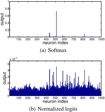
Because a CNN was trained with one-hot hard targets (class labels), given a training image as input, the softmax function suppresses the outputs of most neurons in the output layer and leaves one or a few peak values. For example, in Figure 1 (a), we show the softmax (T = 1) outputs for a training image. To magnify the tiny values in the softmax outputs, after a CNN was trained with softmax function (T = 1), we take the logits y in e.q. (1) and apply the following normalization function
for all i, as the outputs of the CNN, with all the parameters in the CNN unchanged. This function normalizes y so that x in eq. (2) is still a probability distribution over classes. We call the x in eq. (2) normalized logits. In Figure 1 (b), we show the outputs of this function given the same input image as Figure 1 (a).
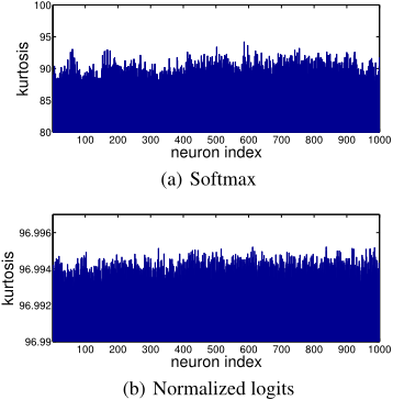
In order to apply ICA, the variables must not all be Gaussian. The non-Gaussianity of a random variable x of zero mean can be measured by kurtosis E(x4 )◁E(x2 )2 -3, which is zero if x is Gaussian. We computed the kurtosis of the outputs (mean removed) of a CNN with softmax and normalized logits using all the ImageNet ILSVRC2012 training data. The CNN model and experimental settings are described in Section 4. The result is, all neurons in the output layer have positive kurtosis, as shown in Figure 2. Therefore the neurons as random variables are highly non-Gaussian and it is sensible to apply ICA, which is introduced in the next section.
3 Factor Analysis
In Factor Analysis, we assume the observed variables x = (x1↪ ▷▷▷↪ xn) are generated by the following model
where s = (s1↪ ▷▷▷↪ sn) are the latent variables, A is the model parameter matrix and n are the noise variables. Here, x and s are assumed to have zero-mean. s are also assumed to be uncorrelated and have unit variance, in other words, white.
3.1 Principle Component Analysis
Principle Component Analysis (PCA) is a special case of Factor Analysis. In PCA, s are assumed to be Gaussian and n are assumed to be zero (noise-free). Let C denote the covariace matrix of x, E = (e1↪ ▷▷▷↪ en) denote the matrix of eigenvectors of C and D = diag(λ1↪ ▷▷▷↪ λn) denote the diagonal matrix of eigenvalues of C. The PCA matrix is ET , the whitening matrix is U = D-1◁2ET and the whitened variables are z = Ux.
3.2 Independent Component Analysis
Independent Component Analysis (ICA) [Hyv¨arinen et al., 2004] is another special case of Factor Analysis. In ICA, s are assumed to be non-Gaussian and independent and n are assumed to be zero. ICA seeks a demixing matrix W such that Wx can be as independent as possible. To obtainW, we can first decompose it as W = VU, where U is the whitening matrix and V is an orthogonal matrix, which can be learned by maximizing the non-Gaussianity or the likelihood function of VUx. The non-Gaussianity can be measured by kurtosis or negentropy. If dimensionality reduction is required, we can take the d largest eigenvalues and the corresponding eigenvectors for the whitening matrix U. As a result, the size of U is d⇥n and the size of V is d⇥d. Scaling each component does not affect ICA solutions. If W is an ICA demixing matrix, then diag(↵1↪ ▷▷▷↪ ↵d)W is also an ICA demixing matrix, where ¶↵1↪ ▷▷▷↪ ↵d♦ are non-zero scaling constants of the components.
A classic ICA algorithm is FastICA [Hyvarinen, 1999]. Despite its fast convergence, FastICA is a batch algorithm which requires all the data to be loaded for computation in each iteration. Thus, it is unsuitable for large scale applications. To handle large scale datasets, we use a stochastic gradient descent (SGD) based ICA algorithm (described in the Appendix of [Hyvarinen, 1999]). For samples ¶z(1)↪ z(2)↪ ▷▷▷♦, one updating step of the SGD-based algorithm of a given sample z(t) is:
where θ is the learning rate, g(·) = -tanh(·) and I is an identity matrix. In our experiments, V was initialized as a random orthogonal matrix.
Like FastICA, this SGD-based algorithm requires going through all data once to compute the whitening matrix U. But unlike FastICA, this SGD-based algorithm does not require projection or orthogonalization in each step.
In this algorithm, the assumption on the probability distribution of each si is a super-Gaussian distribution
and therefore
Since the variables obtained by linear transformations of Gaussian variables are also Gaussian, from Section 2, we can infer at least one neuron in the output layer is non-Gaussian. As an initial attempt, we choose a particular non-Gaussian distribution here. Explorations of different non-Gaussian distributions and therefore different nonlinearities g(·) are left for future research.
4 Results
4.1 Experimental Settings
For the trained CNN model, we used GoogLeNet [Szegedy et al., 2015] and AlexNet [Krizhevsky et al., 2012]. The results of using two different CNN models are similar. Therefore, due to the space limitation, we only report the results of using GoogLeNet. We used all the images in the ImageNet ILSVRC2012 training set to compute the ICA matrix using our SGD-based algorithm with mini-batch size 500. The learning rate was set to 0.005 and was halved every 10 epochs. The computation of CNN outputs was done with Caffe [Jia et al., 2014]. The ICA algorithm was ran with Theano [Bergstra et al., 2010].
4.2 Visualization of PCA/ICA components
To understand what is learned by PCA and ICA, we visualize the PCA and the ICAmatrices. In the PCAmatrix ET or ICA matrix W, each row corresponds to a PCA/ICA component and each column corresponds to an object class. The number of rows depends on the dimensionality reduction. The number of columns of ET or W is 1000, corresponding to 1000 classes. After the ICA matrix was learned, each ICA component (a row of W) was scaled to have unit l2 norm. The scaling of each ICA component does not affect the ICA solution, as discussed in Section 3.2.
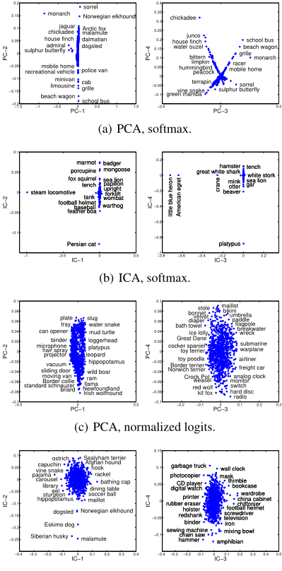
In Figure 3, we show the embedding of class labels by PCA and ICA. The horizontal and the vertical axes are two distinct rows of ET or W. Each point in the plot corresponds to an object class. And there are 1000 points in each plot. Dimensionality is reduced from 1000 to 200 in ICA. In Figure 3 (a) and (b), we plot two pairs of the PCA/ICA components,
(d) ICA, normalized logits.
Figure 3: Label embedding of object class by PCA/ICA components. In each plot, each point is an object class and each axis is a PCA/ICA component (PC/IC). For visual clarity, only selected points are annotated with object class labels.
learned with softmax outputs. In the PCA embedding, visually similar class labels are along some lines, but not the axes, while in the ICA embedding, they are along the axes. However, most points are clustered in the origin. In Figure 3 (c) and (d), we plot two pairs of the PCA/ICA components, learned with normalized logits outputs. We can see the class labels are more scattered in the plots.
In Table 1, we show the top-5 object classes according to the value of PCA/ICA components. For the ease of comparison, we selected each PCA/ICA component which has the largest value for class mosque, killer whale, Model T or zebra among all components. We can see that the class labels ranked by ICA components are more visually similar and consistent than the ones by PCA components.
| 1 | 2 | 3 | 4 | |
|---|---|---|---|---|
| PCA | mosque shoji trimaran fire screen aircraft carrier | killer whale beaver valley otter loggerhead | Model T strawberry hay electric locomotive scoreboard | zebra tiger chickadee school bus yellow lady's slipper |
| ICA | mosque barn planetarium dome palace | killer whale grey whale dugong leatherback turtle sea lion | Model T car wheel tractor disk brake barn | zebra tiger triceratops prairie chicken warthog |
| Egyptian cat | soccer ball | mushroom | red wine | |
|---|---|---|---|---|
| Visual | tabby cat tiger cat tiger lynx Siamese cat | rugby ball croquet ball racket tennis ball football helmet | bolete agaric stinkhorn earthstar hen-of-the-woods | wine bottle beer glass goblet measuring cup wine bottle |
| Semantic | Persian cat tiger cat Siamese cat tabby cat cougar | croquet ball golf ball baseball ping-pong ball punching bag | cucumber artichoke cardoon broccoli cauliflower | eggnog cup espresso menu meat loaf |
The PCA/ICA components can be interpreted as common features shared by visually similar object classes. From Figure 3 and Table 1, we can see the label embeddings of object classes by PCA/ICA components are meaningful since visually similar classes are close in the embeddings. Unlike [Akata et al., 2013], these label embeddings can be unsupervisedly learned with a CNN trained with only one-hot class labels and without any hand annotated attribute label of the object classes, such as has tail or lives in the sea.
4.3 Visual vs. Semantic Similarity
The visual-semantic similarity relationship was previously explored in [Deselaers and Ferrari, 2011], which shows some consistency between two similarities. Here we further explore it from another perspective. We define the visual and the semantic similarity in the following way. The visual similarity between two object classes is defined as cosine similarity of their PCA or ICA components (200-dim and learned with softmax), both of which give the same results. The semantic similarity is defined based on the shortest path length 1 between two classes on the WordNet graph [Fellbaum, 1998].
In Table 2, we compare five closest classes of Egyptian cat, soccer ball, mushroom and red wine in terms of visual and semantic similarities. For Egyptian cat, both visual and semantic similarities give similar results. For soccer ball, football helmet is close in terms of visual similarity but distant in terms of semantic similarity. For mushroom and red wine, two similarities give very different closest object classes. The gap between two similarities is intriguing and therefore worth further exploration. In neuroscience literature, it is claimed that visual cortex representation favors visual rather than semantic similarity [Baldassi et al., 2013].
1 Computed with the path similarity() function in the NLTK tool http://www.nltk.org/howto/wordnet.html.
5 Application: Zero-shot Learning
To demonstrate the effectiveness of the visual features of object classes learned by PCA and ICA, we apply them to zeroshot learning. Zero-shot learning [Larochelle et al., 2008; Lampert et al., 2009; Palatucci et al., 2009] is a classification task in which some classes have no training data at all. We call the classes which have training data seen classes and those which have no training data unseen classes. One can use external knowledge of the classes, such as attributes, to build the relationship between the seen and the unseen classes. Then one can extrapolate the unseen classes by the seen classes.
5.1 Previous Work
The current state-of-the-art large scale zero-shot learning methods are DeViSE [Frome et al., 2013] and conSE [Norouzi et al., 2014]. Both of them use the ImageNet of 1000 classes for training and the ImageNet of over 20000 classes for testing. Our method differs from DeViSE and conSE by using unsupervised learning algorithms to learn: (1) Visual features of classes. (2) Semantic features of classes from the WordNet graph, instead of word2vec [Mikolov et al., 2013] on Wikipedia. (3) A bridge between the visual and the semantic features.
5.2 Our Method
Our method works as follows. In the learning phase, first assume we have obtained the visual feature vectors W(1) = (w(1) 1 ↪ ▷▷▷↪w(1) n ) of n seen classes. Let M = (m1↪ ▷▷▷↪mn) denote the matrix of the mean outputs of a CNN of the seen classes. And F = f(W(1)M) = (f1↪ ▷▷▷↪ fn) are the transformed mean outputs of the seen classes, where f(·) is a nonlinear function. Next, assume we have obtained the semantic feature vectors W(2) = (w(2) 1 ↪ ▷▷▷↪w(2) n ) of n seen classes and W(3) = (w(3) 1 ↪ ▷▷▷↪w(3) m ) of m unseen classes. Due to the visual-semantic similarity gap shown in Section 4.3, we learn a bridge between the visual and the semantic representations of object classes via Canonical Correlation Analysis (CCA) [Hotelling, 1936; Hardoon et al., 2004], which seeks two projection matrices P(1) and P(2) such that
where p(k) i is the i-th column of P(k) and Ckl is a covariance or cross-covariance matrix of ¶f1↪ ▷▷▷↪ fn♦ and/or ¶w(2) 1 ↪ ▷▷▷↪w(2) n ♦.
In the testing phase, when a new image arrives, we first compute its CNN output x. Then for P(1)T (f(W(1)x) - 1n Pi fi), we compute its k closest columns of P(2)T W(2) (seen) and/or P(2)T W(3) (unseen). The corresponding classes of these k columns are the top-k predictions. The closeness is measured by cosine similarity.
For W(1) , we compare random, PCA, and ICA matrices of different dimensionality in our experiments. The random matrices are semi-orthogonal, that is, W(1)W(1)T = I but W(1)W(1)T 6= I. For W(2) and W(3) , we use the feature vectors by running classic Multi-dimensional Scaling (MDS) on a distance matrix of both seen and unseen classes. The distance between two classes is measured by one minus the similarity in Section 4.3. Each column of W(2) andW(3) is subtracted by 1n Pi w(2) i . M is approximated by I and f(·) is the scaling normalization of a vector or each column of a matrix to unit l1 norm. We experimented with softmax with different T and normalized logits as the outputs. The best performance (as in Table 3 and Table 4) was obtained with the softmax (T = 1) output for x but ET andWwere learnt with normalized logits.
5.3 Experiments
Following the zero-shot learning experimental settings of DeViSE and conSE, we used a CNN trained on ImageNet ILSVRC2012 (1000 seen classes), and test our method to classify images in ImageNet 2011fall (20842 unseen classes 2 , 21841 both seen and unseen classes). We use topk accuracy (also called flat hit@k in [Frome et al., 2013; Norouzi et al., 2014]) measure, the percentage of test images in which a method's top-k predictions return the true label.
For the trained CNN model, we experimented with GoogLeNet and AlexNet. Although GoogLeNet outperforms AlexNet on the seen classes, two CNN models in our method perform essentially the same on the zero-shot learning tasks. Due to the space limitation, we only report the results of using GoogLeNet.
The sizes of the matrices in our methods: W(1) is k⇥1000, W(2) is 21632⇥1000,W(3) is 21632⇥20842, P(1) is k⇥k, P(2) is k⇥21632, M is 1000⇥1000 and x is 1000⇥1. We used k = 100↪ 500↪ 900 in our experiments. Although W(2) and W(3) are large matrices, we only need to compute once and store P(2)W(2) and P(2)W(3) of size k⇥1000 and k⇥21632, respectively.
In Table 3, we show the results of the three zero-shot learning methods on the test images selected in [Norouzi et al., 2014]. Same as conSE, our method gives correct or reasonable predictions. In Table 4, we show the results of different methods on ImageNet 2011fall. Our method performs better when using PCA or ICA for the visual features than random features. And our method, especially with PCA or ICA features, achieves superior results on this zero-shot learning task.
The results show that in our method the PCA or ICA matrix as visual features of object classes performs better than a randommatrix. Therefore, these visual features, learned PCA and ICA on the outputs of CNN, are indeed effective for the subsequent tasks. The results also show that PCA and ICA give the essentially same classification accuracy. Therefore, in practice we can use PCA instead of ICA, which has much higher computational costs. A comprehensive discussion on PCA vs. ICA for recognition tasks can be found in [Asuncion Vicente et al., 2007].
The code for reproducing the experiments is in 3 .
6 Discussions
The outputs of a neural network contains rich information. CNN was trained with only one-hot targets, which means we assumed object classes are equally similar and CNN was never informed which classes more similar. However, unsupervised learning on CNN outputs reveals the visual similarity of object classes, which sheds lights on the object representation in CNN. Supervised learning alone cannot deal with unseen classes. With unsupervised learning and external knowledge, we can leverage supervised learning to make reasonable predictions on the unseen classes, that is, zero-shot learning.
2 Since class teddy, teddy bear is missing in ImageNet 2011fall, the correct number of classes is 21841-(1000-1) = 20842 rather than 20841.
3 https://github.com/yaolubrain/ULNNO



| Test Images | DeViSE [Frome et al., 2013] | ConSE [Norouzi et al., 2014] | Our Method |
|---|---|---|---|
| water spaniel tea gown bridal gown, wedding gown spaniel tights, leotards | business suit dress, frock hairpiece, false hair, postiche swimsuit, swimwear, bathing suit kit, outfit | periwig, peruke horsehair wig hound, hound dog bonnet macaque toupee, toupe | |
| heron owl, bird of Minerva, bird of night hawk bird of prey, raptor, raptorial bird finch | ratite, ratite bird, flightless bird peafowl, bird of Juno common spoonbill NewWorld vulture, cathartid Greek partridge, rock partridge | ratite, ratite bird, flightless bird kiwi, apteryx moa elephant bird, aepyornis emu, Dromaius novaehollandiae | |
| elephant turtle turtleneck, turtle, polo-neck flip-flop, thong handcart, pushcart, cart, go-cart | California sea lion Steller sea lion Australian sea lion South American sea lion eared seal | fur seal a eared seal fur seal b guadalupe fur seal Alaska fur seal | |
| golden hamster, Syrian hamster rhesus, rhesus monkey pipe shaker American mink, Mustela vison | golden hamster, Syrian hamster rodent, gnawer Eurasian hamster rhesus, rhesus monkey rabbit, coney, cony | golden hamster, Syrian hamster Eurasian hamster prairie dog, prairie marmot skink, scincid, scincid lizard mountain skink | |
| truck, motortruck skidder tank car, tank automatic rifle, machine rifle trailer, house trailer | flatcar, flatbed, flat truck, motortruck tracked vehicle bulldozer, dozer wheeled vehicle | farm machine cultivator, tiller skidder bulldozer, dozer haymaker, hay conditioner | |
| kernel littoral, litoral, littoral zone, sands carillon Cabernet, Cabernet Sauvignon poodle, poodle dog | dog, domestic dog domestic cat, house cat schnauzer Belgian sheepdog domestic llama, Lama peruana | mastiff alpaca, Lama pacos domestic llama, Lama peruana guanaco, Lama guanicoe Seeing Eye dog |
| Test Set | #Classes | #Images | Method | Top-1 | Top-2 | Top-5 | Top-10 | Top-20 |
|---|---|---|---|---|---|---|---|---|
| Unseen | 20842 | 12.9 million | DeViSE (500-dim) ConSE (500-dim) Our method (100-dim, random) Our method (100-dim, PCA) Our method (100-dim, ICA) Our method (500-dim, random) Our method (500-dim, PCA) Our method (500-dim, ICA) Our method (900-dim, random) Our method (900-dim, PCA) Our method (900-dim, ICA) | 0.8 1.4 1.4 1.6 1.6 1.8 1.8 1.8 1.8 1.8 | 1.4 2.2 2.2 2.7 2.7 2.9 3.0 3.0 3.0 3.0 | 2.5 3.9 3.4 4.6 4.6 5.0 5.2 5.2 5.1 5.2 | 3.9 5.8 4.3 6.4 6.3 6.9 7.3 7.3 7.2 7.3 | 6.0 8.3 5.2 8.6 8.5 8.8 9.6 9.7 9.6 9.7 9.7 |
| 1.8 | 3.0 | 5.2 | 7.3 | |||||
| 21841 | 14.2 million | DeViSE (500-dim) | 0.3 | 0.8 | 1.9 | 3.2 | 5.3 | |
| ConSE (500-dim) | 0.2 | 1.2 | 3.0 | 5.0 | 7.5 | |||
| Our method (100-dim, random) | 6.7 | 8.2 | 10.0 | 11.1 | 12.1 | |||
| Our method (100-dim, PCA) | 6.7 | 8.1 | 10.3 | 12.4 | 14.8 | |||
| Our method (100-dim, ICA) | 6.7 | 8.1 | 10.4 | 12.4 | 14.7 | |||
| Both | Our method (500-dim, random) | 6.7 | 8.5 | 11.2 | 13.4 | 15.6 | ||
| Our method (500-dim, PCA) | 6.7 | 8.5 | 11.4 | 13.7 | 16.3 | |||
| Our method (500-dim, ICA) | 6.7 | 8.5 | 11.4 | 13.7 | 16.3 | |||
| Our method (900-dim, random) | 6.7 | 8.5 | 11.4 | 13.7 | 16.2 | |||
| Our method (900-dim, PCA) | 6.7 | 8.5 | 11.4 | 13.7 | 16.3 | |||
| Our method (900-dim, ICA) | 6.7 | 8.5 | 11.4 | 13.7 | 16.3 |
@inproceedings{ijcai2016p485,
  title     = {Unsupervised Learning on Neural Network Outputs: With Application in Zero-Shot Learning},
  author    = {Lu, Yao},
  booktitle = {Proceedings of the Twenty-Fifth International Joint Conference on
               Artificial Intelligence, {IJCAI-16}},
  publisher = {AAAI Press / International Joint Conferences on Artificial Intelligence},
  editor    = {Subbarao Kambhampati},
  pages     = {3432--3437},
  year      = {2016},
  month     = {7},
  url       = {https://ijcai.org/proceedings/2016/485},
}
TY - CPAPER TI - Unsupervised Learning on Neural Network Outputs: With Application in Zero-Shot Learning AU - Lu, Yao T2 - Proceedings of the Twenty-Fifth International Joint Conference on Artificial Intelligence, IJCAI-16 PB - AAAI Press / International Joint Conferences on Artificial Intelligence PY - 2016 SP - 3432 EP - 3437 UR - https://ijcai.org/proceedings/2016/485 ER -Copied
Machine-readable versions of this paper, for tools and AI agents:





