
On State-Dominance Criteria in Fork-Decoupled Search
Proceedings of the Twenty-Fifth International Joint Conference on Artificial Intelligence. Pages 3265-3270.
© 2016 International Joint Conferences on Artificial Intelligence
Abstract
Fork-decoupled search is a recent approach to classical planning that exploits fork structures, where a single center component provides preconditions for several leaf components. The decoupled states in this search consist of a center state, along with a price for every leaf state. Given this, when does one decoupled state dominate another? Such state-dominance criteria can be used to prune dominated search states. Prior work has devised only a trivial criterion. We devise several more powerful criteria, show that they preserve optimality, and establish their interrelations. We show that they can yield exponential reductions. Experiments on IPC benchmarks attest to the possible practical benefits.
- [Aghighi et al., 2015] Meysam Aghighi, Peter Jonsson, and Simon Ståhlberg. Tractable cost-optimal planning over re- stricted polytree causal graphs. In Blai Bonet and Sven Koenig, editors, Proceedings of the 29th AAAI Confer- ence on Artificial Intelligence (AAAI'15), pages 3225- 3231. AAAI Press, January 2015.
- [Amir and Engelhardt, 2003] Eyal Amir and Barbara Engel- hardt. Factored planning. In G. Gottlob, editor, Proceed- ings of the 18th International Joint Conference on Arti- ficial Intelligence (IJCAI'03), pages 929-935, Acapulco, Mexico, August 2003.
- Morgan Kaufmann. [Bäckström and Nebel, 1995] Christer Bäckström and Bern- hard Nebel. Complexity results for SAS + planning. Com- putational Intelligence, 11(4):625-655, 1995.
- [Brafman and Domshlak, 2003] Ronen Brafman and Carmel Domshlak. Structure and complexity in planning with unary operators. Journal of Artificial Intelligence Re- search, 18:315-349, 2003.
- [Brafman and Domshlak, 2013] Ronen Brafman and Carmel Domshlak. On the complexity of planning for agent teams and its implications for single agent planning. Artificial Intelligence, 198:52-71, 2013.
- [Fabre et al., 2010] Eric Fabre, Loïg Jezequel, Patrik Haslum, and Sylvie Thiébaux. Cost-optimal factored planning: Promises and pitfalls. In Ronen I. Brafman, Hector Geffner, Jörg Hoffmann, and Henry A. Kautz, editors, Proceedings of the 20th International Conference on Automated Planning and Scheduling (ICAPS'10), pages 65-72. AAAI Press, 2010.
- [Gentilini et al., 2003] Raffaella Gentilini, Carla Piazza, and Alberto Policriti. From bisimulation to simulation: Coars- est partition problems. Journal of Automated Reasoning, 31(1):73-103, 2003.
- [Gnad and Hoffmann, 2015] Daniel Gnad and Jörg Hoff- mann. Beating LM-cut with h max (sometimes): Fork- decoupled state space search. In Ronen Brafman, Carmel Domshlak, Patrik Haslum, and Shlomo Zilberstein, edi- tors, Proceedings of the 25th International Conference on Automated Planning and Scheduling (ICAPS'15). AAAI Press, 2015.
- [Helmert and Domshlak, 2009] Malte Helmert and Carmel Domshlak. Landmarks, critical paths and abstractions: What's the difference anyway? In Alfonso Gerevini, Adele Howe, Amedeo Cesta, and Ioannis Refanidis, edi- tors, Proceedings of the 19th International Conference on Automated Planning and Scheduling (ICAPS'09), pages 162-169. AAAI Press, 2009.
- [Helmert, 2006] Malte Helmert. The Fast Downward plan- ning system. Journal of Artificial Intelligence Research, 26:191-246, 2006.
- [Jonsson and Bäckström, 1995] Peter Jonsson and Christer Bäckström. Incremental planning. In European Workshop on Planning, 1995.
- [Katz and Domshlak, 2008] Michael Katz and Carmel Domshlak. Structural patterns heuristics via fork decomposition. In Jussi Rintanen, Bernhard Nebel, J. Christopher Beck, and Eric Hansen, editors, Proceed- ings of the 18th International Conference on Automated Planning and Scheduling (ICAPS'08), pages 182-189. AAAI Press, 2008.
- [Katz and Keyder, 2012] Michael Katz and Emil Keyder. Structural patterns beyond forks: Extending the complex- ity boundaries of classical planning. In Jörg Hoffmann and Bart Selman, editors, Proceedings of the 26th AAAI Con- ference on Artificial Intelligence (AAAI'12), pages 1779- 1785, Toronto, ON, Canada, July 2012. AAAI Press.
- [Kelareva et al., 2007] Elena Kelareva, Olivier Buffet, Jinbo Huang, and Sylvie Thiébaux. Factored planning using de- composition trees. In M. Veloso, editor, Proceedings of the 20th International Joint Conference on Artificial Intel- ligence (IJCAI'07), pages 1942-1947, Hyderabad, India, January 2007. IJCAI
- Morgan Kaufmann. [Knoblock, 1994]
- Craig Knoblock. Automatically gener- ating abstractions for planning. Artificial Intelligence, 68(2):243-302, 1994.
- [Milner, 1971] Robin Milner. An algebraic definition of sim- ulation between programs. In Proceedings of the 2nd In- ternational Joint Conference on Artificial Intelligence (IJ- CAI'71), pages 481-489, London, UK, September 1971. IJCAI
- William Kaufmann. [Torralba and Hoffmann, 2015] Álvaro Torralba and Jörg Hoffmann. Simulation-based admissible dominance prun- ing. In Qiang Yang, editor, Proceedings of the 24th In- ternational Joint Conference on Artificial Intelligence (IJ- CAI'15), pages 1689-1695. AAAI Press/IJCAI, 2015. IJCAI
- [Torralba and Kissmann, 2015] Álvaro Torralba and Peter Kissmann. Focusing on what really matters: Irrelevance pruning in merge-and-shrink. In Levi Lelis and Roni Stern, editors, Proceedings of the 8th Annual Symposium on Combinatorial Search (SOCS'15), pages 122-130. AAAI Press, 2015.
References were extracted automatically from the PDF and may contain errors.
Full text extracted automatically from the PDF; figures, tables and equations may differ. The PDF is the version of record.
1 Introduction
Fork-decoupled search is a new approach to state-space decomposition in classical planning, recently introduced by Gnad and Hoffmann [2015]. The approach partitions the state variables into disjoint subsets, factors, like in factored planning (e. g. [Amir and Engelhardt, 2003; Kelareva et al., 2007; Fabre et al., 2010; Brafman and Domshlak, 2013]). While factored planning is traditionally designed to handle arbitrary cross-factor interactions, fork-decoupling assumes these interactions to take a fork structure [Katz and Domshlak, 2008; Katz and Keyder, 2012; Aghighi et al., 2015], where a single center provides preconditions for several leaves. A simple pre-process can determine whether such a fork structure exists, and extract a corresponding factoring if so.
Fork factorings identify a form of "conditional independence" between the leaf factors: Given a fixed center path ⇡C , the compliant leaf moves - those leaf moves enabled by the preconditions supplied along ⇡C - can be selected independently for each leaf. The decoupled search thus searches only over center paths ⇡C . Each decoupled state in the search represents the compliant leaf moves in terms of a pricing function, mapping each leaf-factor state sL to the cost of a cheapest ⇡C -compliant path achieving sL. As Gnad and Hoffmann (henceforth: GH) show, this can exponentially reduce state space size. It may also cause exponential blow-ups though.
The worst-case exponential blow-ups result from irrelevant distinctions in pricing functions. One means to combat this, and more generally to improve search, is dominance pruning, pruning a state sF if a better state tF has already been seen. But, given the complex structure of decoupled states, when is one "better" than another? GH employ the trivial criterion, where sF and tF must have the same center state and tF needs to have cheaper prices than sF for all leaf states. Here we introduce advanced methods, analyzing the structure of decoupled states to identify (and then, disregard) irrelevant distinctions. We devise several such methods, using different sources of information. We show that the methods preserve optimality, and we characterize their relative pruning power. We show that they can yield exponential search reductions. Experiments on International Planning Competition (IPC) benchmarks attest to the possible practical benefits.
For space reasons, we can only outline our proof arguments. Full proofs will be made available in an online TR.
2 Background
We use finite-domain state variables [B¨ackstr¨om and Nebel, 1995; Helmert, 2006]. A planning task is a tuple ⇧ = hV↪A↪ I↪Gi. V is a set of variables, each associated with a finite domain D(v). I is the initial state. The goal G is a partial assignment to V. A is a finite set of actions, each a triple hpre(a)↪ e↵(a)↪ cost(a)i of precondition, effect, and cost, where pre(a) and e↵(a) are partial assignments to V, and cost(a) 2 R0+. For a partial assignment p, we denote with V(p) ✓ V the subset of variables on which p is defined. For V ✓ V(p), we denote with p[V ] the assignment to V made by p. We identify (partial) variable assignments as sets of variable/value pairs, written as (var, val). A state is a complete assignment to V. Action a is applicable in state s if pre(a) ✓ s. Applying a in s changes the value of all v 2 V(e↵(a)) to e↵(a)[v], and leaves s unchanged elsewhere. We will sometimes write s a-! t for a transition from s to t with action a. A plan for ⇧ is an action sequence ⇡ iteratively applicable in I which results in a state sG where G ✓ sG. The plan is optimal if its summed-up cost, denoted cost(⇡), is minimal among all plans for ⇧.
We next give a recap of GH's definitions. A fork factoring F is a partition of V identifying a fork structure. Namely, (i) every action a 2 A affects (touches in its effect) exactly one element (factor) of F, which we denote F(a). And (ii) there is a center F C 2 F s.t., for every a 2 A, V(pre(a)) ✓
F C [ F(a). We refer to the factors F L 2 F L := F ∩ ¶F C ♦ as leaves. We refer to actions affecting F C as center actions, and to actions affecting a leaf as leaf actions. By construction (each action affects only one factor) these two kinds of actions are disjoint. Center actions are preconditioned only on F C , leaf actions may be preconditioned on F C and the leaf they affect. In brief: the center provides preconditions for the leaves, and there are no other cross-factor interactions.
As a running example, we use a Logistics-style planning task with a truck variable t, a package variable p, and n locations l1↪ ▷ ▷ ▷ ↪ ln. I = ¶(t↪ l1)↪ (p↪ l1)♦ and G = ¶(p↪ l2)♦. Action drive(x↪ y) moves the truck from any location x to any other location y. The package can be loaded/unloaded at any location x with actions load(x)/unload(x) respectively. Then F = ¶¶t♦↪ ¶p♦♦ is a fork factoring where ¶t♦ is the center and ¶p♦ is the single leaf. If we have m packages pi, we can set each ¶pi♦ as a leaf.
Not every task ⇧ has a fork factoring. GH analyze ⇧'s causal graph (e. g. [Knoblock, 1994; Jonsson and B¨ackstr¨om, 1995; Brafman and Domshlak, 2003; Helmert, 2006]) in a pre-process, identifying a fork factoring if one exists, else abstaining from solving ⇧. We follow this approach here. In what follows, we assume a fork factoring F. Variable assignments to F C are called center states, and for each F L 2 F L assignments to F L are leaf states. We denote by SL the set of all leaf states, across F L 2 F L. For each leaf, sLI denotes the initial leaf state. For simplicity (wlog), we will assume that every leaf has a single goal leaf state, sLG.
Decoupled search searches over sequences of center actions ⇡C , called center paths, that are applicable to I. For each ⇡C , it maintains a compact representation of the leaf paths ⇡L that comply with ⇡C . A leaf path is a sequence of leaf actions applicable to I when ignoring preconditions on F C . Intuitively, given the fork structure, a fixed center path determines what each leaf can do (independently of all other leaves, as they interact only via the center). This is captured by the notion of compliance: ⇡L complies with ⇡C if it uses only the center preconditions supplied along ⇡C , i. e., if ⇡L can be scheduled alongside ⇡C s.t. the combined action sequence is applicable in I. Decoupled search goes forward from I until it finds a center path ⇡C to a center goal state where every leaf has a ⇡C -compliant leaf path ⇡L to its goal leaf state. The global plan then results from augmenting ⇡C with the paths ⇡L.
In detail: A decoupled state sF is given by a center path cp(sF ). Its center state cs(sF ) and pricing function prices(sF ) : SL 7! R0+ are induced by cp(sF ), as follows. cs(sF ) is the outcome of applying cp(sF ) to sLI . prices(sF ) maps each leaf state sL to the cost of a cheapest cp(sF )- compliant leaf path ending in sL (or 1 if no such path exists). 1 The initial decoupled state I F has the empty center path cp(I F ) = hi. A goal decoupled state sFG is one with a goal center state cs(sFG ) ◆ G[F C ] and where, for every leaf factor F L 2 F L, its goal leaf state sLG has been reached, i. e., prices(sFG )[sLG] <1. The actions applicable in sF are those center actions a where pre(a) ✓ cs(sF ). Applying a to sF
1 Pricing functions can be maintained in time low-order polynomial in the size of the individual leaf state spaces. See GH for details.
results in tF where cp(tF ) := cp(sF ) ◦ hai, inducing cs(tF ) and prices(tF ) as above.
In the running example, cs(I F ) = ¶(t↪ l1)♦, prices(I F )[(p↪ l1)] = 0, prices(I F )[(p↪ t)] = 1, and prices(I F )[(p↪ li)] = 1, for all i 6= 1. Observe that prices(I F )[(p↪ t)] represents the cost of a possible package move, not a move we have already committed to. The actions applicable to I F are drive(l1↪ li). Applying any such action, in the outcome decoupled state sF we have prices(sF )[(p↪ li)] = 2, while all other prices remain the same. If we apply drive(l1↪ l2), then sF is a goal decoupled state. The global plan is then extracted from sF by augmenting the center path cp(sF ) = hdrive(l1↪ l2)i with the compliant goal leaf path hload(l1)↪unload(l2)i.
A completion plan for sF consists of a center path ⇡C leading from sF to some goal center state, augmented with goal leaf paths compliant with cp(sF ) ◦ ⇡C . That is, we collect the postfix path for the center, and the complete path for each leaf. The completion cost of sF , denoted hF⇤ (sF ), is defined as the cost of a cheapest completion plan for sF . By dF⇤ (sF ), we denote the minimum, over all optimal completion plans ⇡F , of the number of center actions (decoupled-state transitions) in ⇡F .
3 Decoupled State Dominance
A binary relation ⪯ over decoupled states is a decoupled dominance relation if sF ⪯ tF implies that hF⇤ (sF ) ≥ hF⇤ (tF ) and dF⇤ (sF ) ≥ dF⇤ (tF ). In dominance pruning, given such a relation ⪯, we prune a state sF at generation time if we have already seen another state tF (i. e., tF is in the open or closed list) such that sF ⪯ tF and g(sF ) ≥ g(tF ). Intuitively, tF dominates sF if it has an at least equally good completion plan and center path. The center path condition is needed only in the presence of 0-cost actions, and ensures that the completion plan for tF does not have to traverse sF . If tF can be reached with equal or better g-cost, pruning sF preserves completeness and optimality of the search algorithm.
We derive practical decoupled dominance relations by efficiently testable sufficient criteria. The relations differ in terms of their pruning power. We capture their relative power with two simple terms of two simple notions. First, we say that ⪯0 subsumes ⪯ if ⪯0◆⪯, i. e., if ⪯0 recognizes every occurrence of dominance recognized by ⪯. Second, we say that ⪯0 is exponentially separated from⪯ if there exists a family of planning tasks in which the decoupled state space is exponential in the size of the input task under dominance pruning using ⪯ and polynomial when using ⪯0 . 2 We will devise several decoupled dominance relations, weaker and stronger ones. Weaker relations are useful in practice (only) when they cause less computational overhead.
Previous work only considered what we will refer to as the basic decoupled dominance relation, denoted ⪯B.
Definition 1 (⪯B relation) ⪯B is the relation over decoupled states defined by sF ⪯B tF iff cs(sF ) = cs(tF ) and, for all sL 2 SL, prices(sF )[sL] ≥ prices(tF )[sL].
2 More precisely, as the pruning depends on the expansion order: in which this statement is true for any expansion order.
This method simply does a point-wise comparison between prices(sF ) and prices(tF ), whenever both have the same center state. Basic dominance pruning often helps to reduce search effort, but is unnecessarily restrictive in its insistence on all leaf prices being cheaper. This is inappropriate in cases where sF has some irrelevant cheaper prices. It may, indeed, cause exponential blow-ups as, e. g., in our running example.
The standard state space in our running example is small, since ♣V♣ = 2. Yet the decoupled state space has size exponential in the number n of locations. Through the leaf state prices, the decoupled states "remember" the locations visited by the truck in the past. For example, the decoupled state reached through the center sequence hdrive(l1↪ l3)↪ drive(l3↪ l4)i has finite prices for (p↪ l1), (p↪ t), (p↪ l3), and (p↪ l4), and price 1 elsewhere; while the decoupled state reached through the sequence hdrive(l1↪ l4)i has finite prices for (p↪ l1), (p↪ t), and (p↪ l4). Intuitively, the difference between the two pricing functions does not matter, because, with initial location l1 and goal location l2, the prices for (p↪ li)↪ i > 2 are irrelevant. But without recognizing this fact, the decoupled state space enumerates (pricing functions corresponding to) every combination of visited locations.
It is remarkable here that the blow-up occurs in a simple Logistics task. This is a new insight. GH already pointed out the risk of blow-ups, but only in complex artificial examples. On IPC benchmarks, empirically the decoupled state space always is smaller than the standard one. Our insight here is that this is not because blow-ups don't occur, but because the blow-ups (e. g. remembering truck histories) are hidden behind the gains (e. g. not enumerating combinations of package locations). Indeed, in the standard IPCLogistics benchmarks, the blow-up above occurs for all non-airport locations within every city, and these blow-ups multiply across cities. All our advanced dominance pruning methods get rid of this blow-up (though none guarantees to avoid blow-ups in general).
4 Frontier-Based Dominance
Our first dominance relation is based on the idea that differing prices on a leaf state sL do not matter if "sL has no purpose". In our running example, say that we are checking whether sF ⪯ tF and prices(sF )[(p↪ l3)] = 2 while prices(tF )[(p↪ l3)] = 1, and thus sF 6⪯B tF . However, say that prices(sF )[(p↪ t)] = 1. Then the cheaper price for (p↪ l3) in sF does not matter, because the only purpose of having the package at l3 is to load it into the truck. Indeed, the only outgoing transition of the leaf state (p↪ l3) leads to (p↪ t).
We capture the relevant leaf states in sF in terms of its frontier: those leaf states that are either themselves relevant (this applies only to the goal leaf state), or that can still contribute to achieving cheaper prices somewhere.
Definition 2 (Frontier) We define the frontier of a decoupled state sF , F(sF ) ✓ SL as F(sF ) := ¶sLG♦ [ ¶sL ♣ 9sL a-! tL : prices(sF )[sL] + cost(a) < prices(sF )[tL]♦.
We now obtain a decoupled dominance relation by comparing prices only on the frontier of sF :
Definition 3 (⪯F relation) ⪯F is the relation over decoupled states defined by sF ⪯F tF iff cs(sF ) = cs(tF ) and, for all sL 2 F(sF ), prices(sF )[sL] ≥ prices(tF )[sL].
Theorem 1 ⪯F is a decoupled dominance relation.
Comparing the prices on the frontier is enough because, in any completion plan for sF , if a compliant leaf path ⇡L decreases the price of the goal leaf state (e. g., from 1 to some finite value), then ⇡L must pass through a frontier state sL. Hence, in a completion plan for tF , we can use the postfix behind sL. This completion plan can only be better than that for sF because prices(sF )[sL] ≥ prices(tF )[sL].
Theorem 2 ⪯F subsumes ⪯B and is exponentially separated from it.
It is easy to see that ⪯F is strictly better than ⪯B:
The first part of this claim is trivial as both relations are based on comparing prices, but ⪯F does so on a subset of leaf states. A task family demonstrating the second part of the claim is our running example. The only leaf action applicable in any leaf state (p↪ li) is load(li), leading to (p↪ t). However, for any reachable sF , we have prices(sF )[(p↪ t)] = 1 because this price is already achieved in the initial state, and prices can only decrease. So the only possible frontier state, apart from (p↪ t), is the goal (p↪ l2). But only two different prices are reachable for (p↪ l2), namely 1 and 2. This shows the claim.
5 Effective-Price Dominance
Our next method appears orthogonal to frontier-based dominance at first sight, but turns out to subsume it. The method is based on replacing the prices in tF , i. e., the dominating state in the comparison sF ⪯ tF , with smaller effective prices, denoted Eprices(tF ). We then simply compare all such prices:
Definition 4 (⪯E relation) ⪯E is the relation over decoupled states defined by sF ⪯E tF iff cs(sF ) = cs(tF ) and, for all sL 2 SL, prices(sF )[sL] ≥ Eprices(tF )[sL].
The modified comparison is sound because the effective prices are designed to preserve hF⇤ (tF ). Precisely: (*) For any center path ⇡C starting in tF , and for any leaf state sL of leaf F L, if ⇡L s is a ⇡C -compliant leaf path from sL to sLG, then there exists a path ⇡L from sLI to sLG that complies with cp(tF ) ◦ ⇡C such that cost(⇡L) Eprices(tF )[sL] + cost(⇡L s ). In other words, if prices(tF )[sL] > Eprices(tF )[sL], then any completion plan can be modified to use some other leaf state which does provide a total price of Eprices(tF )[sL] + cost(⇡L s ) or less.
It turns out that this can be ensured with the following simple definition. We define Eprices(tF ) as the point-wise minimum pricing function p that satisfies:
For each F L, Eprices(tF ) can be computed by a simple backwards algorithm starting at the goal leaf state sLG. To illustrate the definition, consider any tF in our running example. The price of (p↪ t) is 1, and its effective price also is 1 because its successor leaf state sLG = (p↪ l2) always has effective price ≥ 2. For any irrelevant location li, i > 2, however, due to the transition to (p↪ t) whose effective price is 1, we get Eprices(tF )[(p↪ li)] = 0 regardless of what the actual price
of (p↪ li) in tF is. The effective price 0 is sound because, in any completion plan for tF starting with load(li), we can use load(l1) instead to get (p↪ t) with price 1.
Theorem 3 ⪯E is a decoupled dominance relation.
Formally, denote ⇡L s = ha1↪ ▷ ▷ ▷ ↪ ani and denote the leaf states it traverses by sL = sL0 ↪ ▷ ▷ ▷ ↪ sLn = sLG. Observe that, as Eprices(tF )[sLn ] = prices(tF )[sLn ], ⇡L s necessarily passes through a leaf state sLi whose effective and actual prices in tF are identical. Let i be the smallest index for which that is so. Then, for all j < i, Eprices(tF )[sLj ] 6= prices(tF )[sLj ], and thus by the definition of effective prices we have that Eprices(tF )[sLj ] ≥ Eprices(tF )[sLj+1 ] - cost(aj+1). Accumulating these inequalities, we get (**) Eprices(tF )[sL0 ] ≥ Eprices(tF )[sLi ] - Pij=1 cost(aj). Consider now the path ⇡L from sLI to sLG constructed as the concatenation of: a cheapest cp(tF )-compliant path to sLi (in our example, hload(l1)); with the postfix of ⇡L s behind sLi (in our example, hunload(l2)). Then cost(⇡L) = prices(tF )[sLi ] + Pnj=i+1 cost(aj). As Eprices(tF )[sLi ] = prices(tF )[sLi ], we get cost(⇡L) = Eprices(tF )[sLi ] + Pnj=i+1 cost(aj). With (**), we get the desired property that cost(⇡L) Eprices(tF )[sL0 ] + Pij=1 cost(aj) + Pnj=i+1 cost(aj) = Eprices (tF )[sL] + cost(⇡L s ), concluding the proof.
To prove Theorem 3, observe that, whenever sF ⪯E tF , given a completion plan for sF , we can construct an equally good completion plan for tF by using the same center path ⇡C , and, with (*) above, constructing equally good or cheaper compliant goal leaf paths. It remains to prove (*). Consider any tF , center path ⇡C , leaf state sL, and ⇡C -compliant goal leaf path ⇡L s starting in sL. In our example, e. g., say tF is reached from I F by applying drive(l1↪ l3); that ⇡C = hdrive(l3↪ l2)i; that sL = (p↪ l3); and that ⇡L s = hload(l3)↪ unload(l2)i. Then, exists ⇡L = hload(l1)↪ unload(l2)i that is compliant with cp(tF ) ◦ ⇡C .
Theorem 4 ⪯E subsumes ⪯F and is exponentially separated from it.
To prove the exponential separation, we extend our running example with a teleport(li↪ lj) action, for i↪ j > 2, that moves the package between irrelevant locations if the truck is at l2. Then, as long as l2 and at least one such li have not been visited yet, all leaf states (p↪ li) for i > 2 with finite price are in the frontier, and ⪯F suffers from the same blow-up as ⪯B. The effective prices of (p↪ li), however, remain 0 as before.
To see that ⪯E subsumes ⪯F , observe that the former can be viewed as a recursive version of the latter, when reformulating the frontier condition to "9sL a-! tL : p[sL] < p[tL] - cost(a)". Formally, one can show that, if Eprices(tF )[sL] prices(sF )[sL] holds for all frontier states sL 2 F(sF ), then it also holds for all non-frontier states sL 62 F(sF ). This shows the claim as, for sF ⪯F tF , we have prices(sF )[sL] ≥ prices(tF )[sL] on sL 2 F(sF ), and thus prices(sF )[sL] ≥ Eprices(tF )[sL] on these states.
Note that, with the above, to evaluate ⪯E it suffices to compare the price of sF vs. effective price of tF on F(sF ). This is equivalent to, but faster than, comparing all prices.
6 Simulation-Based Dominance
We use the concept of simulation relations [Milner, 1971; Gentilini et al., 2003] on leaf state spaces in order to identify leaf states tL which can do everything that another leaf state sL can do. 3 In this situation, suppose that we are checking whether sF ⪯ tF , and prices(tF )[sL] > prices(sF )[sL], but prices(tF )[tL] prices(sF )[sL]. Then tF can still dominate sF , because if a solution for sF relies on sL, then starting from tF we can use tL instead.
Definition 5 (Leaf simulation) Let F L be a leaf factor. A binary relation ⪯L on F L leaf states is a leaf simulation if: sLG 6⪯L sL for all sL 6= sLG; and whenever sL1 ⪯L tL1 , for every transition sL1 a-! sL2 either (i) sL2 ⪯L tL1 or (ii) there exists a transition tL1 a0 -! tL2 s.t. sL2 ⪯L tL2 , pre[F C ](a0 ) ✓ pre[F C ](a), and cost(a0 ) cost(a).
This follows common notions, except for (i) which, intuitively, "allows tL1 to stay where it is", and except for allowing in (ii) different actions a0 so long as they are at least as good in terms of center precondition and cost.
It is easy to see that, whenever sL ⪯L tL, if a leaf path ⇡L s starting in sL complies with a center path ⇡C , then there exists a ⇡C -compliant leaf path ⇡L t starting in tL s.t. cost(⇡L t ) cost(⇡L s ). Consequently, we allow sL to take a cheaper price from any leaf state that simulates it:
Definition 6 (⪯S Relation) The relation ⪯S over decoupled states is defined by sF ⪯S tF iff cs(sF ) = cs(tF ) and, for all sL 2 SL, prices(sF )[sL] ≥ minsL⪯L tL prices(tF )[tL].
Theorem 5 ⪯S is a decoupled dominance relation.
Theorem 6 ⪯S subsumes ⪯B and is exponentially separated from it.
It is easy to see that this is strictly better than ⪯B:
The first part of this claim holds simply because ⪯L is reflexive (and therefore minsL⪯L tL prices(tF )[tL] prices(tF )[sL]). For the second part, we use again our running example. Leaf simulation captures that (p↪ li) ⪯L (p↪ t) for all i > 2, since (p↪ t) is the only successor of any (p↪ li) and naturally (p↪ t) ⪯L (p↪ t). So, ⪯S reduces the price of such (p↪ li) to 1, avoiding the exponential blow-up.
Inspired by [Torralba and Kissmann, 2015], we also employ leaf simulation to remove superfluous leaf states and leaf actions, discovering transitions that can be replaced by other transitions, then running a reachability check on the leaf state space (details are in the TR). This reduces leaf state space size, and may sometimes improve the heuristic function due to the removal of some actions.
7 Method Interrelations and Combination
We have already established the relation of our methods relative to ⪯B, as well as the relation between ⪯E and ⪯F . We next design a combination ⪯ES of ⪯E and ⪯S, with their respective strengths, and we establish the remaining method interrelations. Figure 1 provides the overall picture.
3 This is inspired by, but differs in scope and purpose from, the use of simulation relations on the state space for dominance pruning in standard search [Torralba and Hoffmann, 2015].
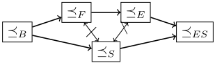
The combined relation ⪯ES is obtained by modifying the effective prices underlying ⪯E, enriching their definition with a leaf simulation, ⪯L. We define ESprices(tF ) as the point-wise minimum pricing function p that satisfies:
We integrate the information from a leaf simulation into the effective prices by allowing sL to take cheaper prices from simulating states tL. This amounts to substituting prices(tF )[sL] with minsL⪯L tL prices(tF )[tL] in the equation. We thus obtain, again, a decoupled dominance relation:
Definition 7 (⪯ES Relation) ⪯ES is the relation over decoupled states defined by sF ⪯ES tF iff cs(sF ) = cs(tF ) and, for all sL 2 SL, prices(sF )[sL] ≥ ESprices(tF )[sL].
Theorem 7 is shown by adapting the property (*) underlying the proof of Theorem 3. Say ⇡L s = ha1↪ ▷ ▷ ▷ ↪ ani is a ⇡C -compliant goal leaf path starting in sL, traversing the leaf states sL = sL0 ↪ ▷ ▷ ▷ ↪ sLn = sLG. Then, with the same arguments as before, there exists i such that (a) ESprices(tF )[sL0 ] ≥ ESprices(tF )[sLi ] - Pij=1 cost(ai), and (b) ESprices(tF )[sLi ] = minsLi ⪯L tL prices(tF )[tL]. We construct our desired path ⇡L from sLI to sLG by a cheapest cp(tF )-compliant path to a tL minimizing the expression in (b), concatenated with a ⇡C -compliant goal leaf path ⇡L t starting in tL where cost(⇡L t ) cost(⇡L s ). Such ⇡L t exists by the properties of leaf simulation, as in Theorem 5.
Theorem 7 ⪯ES is a decoupled dominance relation.
⪯ES subsumes each of its components. The exponential separations therefore follow directly from the individual ones:
Theorem 8 ⪯ES subsumes ⪯E and ⪯S, and is exponentially separated from each of them.
One can also construct cases where ⪯ES yields an exponentially stronger reduction than both ⪯E and ⪯S , i. e., where ⪯ES is strictly more than the sum of its components. We complete our analysis by filling in the missing cases:
Theorem 9 ⪯S is exponentially separated from ⪯E, and therefore also from ⪯F . ⪯F , and therefore also ⪯E, is exponentially separated from ⪯S.
8 Experiments
We implemented our dominance pruning methods within the fork-decoupled search variant of FD [Helmert, 2006] by GH. Our baseline is GH's basic pruning ⪯B. For simplicity, we stick to the factoring strategy used by GH. This method greedily computes a factoring that maximizes the number of leaf factors. In case there are less than two leaves, the method abstains from solving a task. The rationale behind this is that the main advantage of decoupled search originates from not having to enumerate leaf state combinations across multiple leaf factors. Like GH, we show results on all IPC domains up to and including 2014 where the strategy does not abstain.
We focus on optimal planning, the main purpose of optimality-preserving pruning. We run a blind heuristic to identify the influence of different pruning methods per se, and we run LM-cut [Helmert and Domshlak, 2009] as a stateof-the-art heuristic. GH introduced two decoupled variants of A⇤ , "Fork-Decoupled" A⇤ and "Anytime Fork-Root" A⇤ , which to simplify terminology we will refer to as Decoupled A⇤ (DA⇤ ) and Anytime Decoupled A⇤ (ADA⇤ ). DA⇤ is a direct application of A⇤ to the decoupled state space. ADA⇤ orders the open list based on the heuristic estimate of remaining center-cost, uses the heuristic estimate of remaining globalcost for pruning against the best solution so far, and runs until the open list is empty. Both algorithms result in similar coverage, with moderate differences in some domains. Our techniques turn out to be more beneficial for ADA⇤ , which tends to have larger search spaces but less per-node runtime than DA⇤ . We show detailed data for ADA⇤ , and include data for baseline DA⇤ (with ⪯B) for comparison. All experiments are run on a cluster of Intel E5-2660 machines running at 2.20 GHz, with time (memory) cut-offs of 30 minutes (4 GB).
| Blind Heuristic ADA⇤ | LM-cut DA⇤ ADA⇤ | |||||||||||
|---|---|---|---|---|---|---|---|---|---|---|---|---|
| Domain | # | ⪯B | ⪯F | ⪯E | ⪯S | ⪯ES | ⪯B | ⪯B | ⪯F | ⪯E | ⪯S | ⪯ES |
| Driverlog | 20 | 11 | 11 | 11 | 11 | 11 | 13 | 13 | 13 | 13 | 13 | 13 |
| Logistics00 | 28 | 22 | 22 | 22 | 22 | 22 | 28 | 25 | 25 | 27 | 26 | 28 |
| Logistics98 | 35 | 4 | 4 | 5 | 5 | 5 | 6 | 6 | 6 | 6 | 6 | 6 |
| Miconic | 145 | 36 | 45 | 45 | 45 | 45 | 135 | 135 | 135 | 135 | 135 | 135 |
| NoMystery | 20 | 17 | 20 | 20 | 20 | 20 | 20 | 20 | 20 | 20 | 20 | 20 |
| Pathways | 29 | 3 | 3 | 3 | 3 | 3 | 4 | 4 | 4 | 4 | 4 | 4 |
| Rovers | 40 | 7 | 6 | 6 | 7 | 6 | 9 | 9 | 9 | 9 | 9 | 9 |
| Satellite | 36 | 6 | 6 | 6 | 6 | 5 | 7 | 9 | 9 | 8 | 9 | 9 |
| TPP | 27 | 23 | 23 | 22 | 23 | 22 | 18 | 23 | 23 | 22 | 22 | 22 |
| Woodwork08 | 13 | 5 | 5 | 5 | 5 | 5 | 10 | 11 | 11 | 11 | 11 | 11 |
| Woodwork11 | 5 | 1 | 1 | 1 | 1 | 1 | 4 | 5 | 5 | 5 | 5 | 5 |
| Zenotravel | 20 | 11 | 11 | 12 | 12 | 12 | 13 | 11 | 11 | 12 | 12 | 13 |
| 418 | 146 | 157 | 158 | 160 | 157 | 267 | 271 | 271 | 272 | 272 | 275 | |
P 418 146 157 158 160 157 267 271 271 272 272 275
Table 1: Coverage data.
Table 1 shows the number of instances solved, comparing to both baselines DA⇤ and ADA⇤ . Data for DA⇤ with the blind heuristic is not shown as it is identical to that for ADA⇤ . The main gain for blind search stems from Miconic (+9), and NoMystery (+3). When using LM-cut, the advantage over ⪯B is much smaller. We still gain +3 (+2) instances in Logistics00 (Zenotravel). In Satellite and TPP, we lose 1 instance in some configurations due to overhead at no search space reduction. ⪯ES reliably removes the disadvantages of ADA⇤ relative to DA⇤ , and is best in the overall. We never strictly improve coverage over both baselines, though. As we shall see below, this is due to benchmark scaling, i. e., there are domains where runtime is improved over both baselines.
We next analyze the search space size reduction (top part of Table 2). In general, the blind heuristic has more margin of improvement except in Logistics98, where the improvement with LM-cut gets magnified due to the relevance analysis performed when enabling ⪯S. In that domain, removing irrelevant leaf states and leaf actions renders LM-cut a lot stronger. 4 Regarding the relative behavior of pruning techniques, in two domains, namely Miconic and NoMystery, already the simplest technique (⪯F ) gets the maximal improvement factor. In four domains, enabling effective-price pruning on top of frontier pruning results in additional pruning. Combining all techniques in ⪯ES always inherits the strongest search space reduction of its components and in Logistics with LM-cut, it often is strictly better.
| Expansions with Blind Heuristic: Improvement |
|---|
Consider now runtime, Table 2 bottom. One key observation is that, whenever the search space is reduced, the same holds for runtime, even for small search space reduction factors like, e. g., in Zenotravel. Remarkably, in some domains (e. g. Woodworking) where no search reduction is obtained, runtime decreases nevertheless for some simple methods such as ⪯F . This is due to the cheaper dominance check - prices are compared only on frontier leaf states. There are also some bad cases, though, mainly in TPP, but also in Pathways, Rovers, and Satellite. These are also the domains in which coverage slightly decreases. What makes these domains special is the structure of their leaf state spaces. In Pathways, Rovers, and Satellite, all leaves are single variables with a single transition, sLI ! sLG, so there is no room for improvement. In TPP, the leaf state spaces are quite large (up to 5000 states), so our methods incur substantial overhead, but are unable to perform pruning. Presumably, this is because most of the leaf states can play a role in optimally reaching the goal.
4 It may be surprising that, elsewhere, the improvements in Logistics are moderate, despite the inherent blow-up we explained earlier. This is because, in the commonly solved instances, the number of non-airport locations in each city is very small, mostly 1.
Coming back to our previous observation that coverage is never improved over both baselines, the runtime analysis reveals an improvement over both baselines in several domains. ADA⇤ with ⪯S is faster than DA⇤ with ⪯B in all domains except Zenotravel, where the geomean per-instance runtime factor is 0▷7. The other factors are: Driverlog 2▷3; Logistics00 2▷3; Logistics98 3▷4; Miconic 2▷7; NoMystery 3▷2; Pathways 1▷1; Rovers 2▷1; Satellite 2▷9; TPP 23▷2; Woodworking08 1▷4; and Woodworking11 2▷0. In particular, in Driverlog, both Logistics domains, NoMystery, and Woodworking11, ADA⇤ with ⪯S improves runtime over both baselines.
Finally, consider the use of our pruning methods in DA⇤ . For blind search, the numbers are almost identical to those for ADA⇤ in Table 2, as DA⇤ and ADA⇤ differ mainly in their use of a (non-trivial) heuristic. With LM-cut, the pruning methods do not work as well for DA⇤ . For example, for ⪯S, the geomean per-instance runtime factors are: Driverlog 1▷8; Logistics00 and Logistics98 2▷5; NoMystery 2▷0; TPP 0▷9; Woodworking08 0▷9; Woodworking11 1▷3; Zenotravel 1▷2; and 1▷0 in the other domains. The picture is similar for the other pruning methods. The big runtime advantages observed with ADA⇤ vanish, but the method also becomes less risky, i. e., the big runtime disadvantage in TPP vanishes as well. This makes sense since DA⇤ searches less nodes (it has less potential for pruning) while spending more time on each node (making the dominance-checking overhead less pronounced).
9 Conclusion
Dominance pruning methods can be quite useful for decoupled search. Our analysis of such methods is fairly complete, although of course other variants may be thinkable. More pressingly, the question remains whether there exist duplicate checking methods guaranteeing to avoid all blow-ups.
Acknowledgments
This work was partially supported by the German Research Foundation (DFG), under grant HO 2169/6-1, "StarTopology Decoupled State Space Search".
@inproceedings{ijcai2016p462,
  title     = {On State-Dominance Criteria in Fork-Decoupled Search},
  author    = {de Reyna, Álvaro Torralba Arias and Gnad, Daniel and Dubbert, Patrick and Hoffmann, Jörg},
  booktitle = {Proceedings of the Twenty-Fifth International Joint Conference on
               Artificial Intelligence, {IJCAI-16}},
  publisher = {AAAI Press / International Joint Conferences on Artificial Intelligence},
  editor    = {Subbarao Kambhampati},
  pages     = {3265--3270},
  year      = {2016},
  month     = {7},
  url       = {https://ijcai.org/proceedings/2016/462},
}
TY - CPAPER TI - On State-Dominance Criteria in Fork-Decoupled Search AU - de Reyna, Álvaro Torralba Arias AU - Gnad, Daniel AU - Dubbert, Patrick AU - Hoffmann, Jörg T2 - Proceedings of the Twenty-Fifth International Joint Conference on Artificial Intelligence, IJCAI-16 PB - AAAI Press / International Joint Conferences on Artificial Intelligence PY - 2016 SP - 3265 EP - 3270 UR - https://ijcai.org/proceedings/2016/462 ER -Copied
Machine-readable versions of this paper, for tools and AI agents:





