Learning Predictive State Representations via Monte-Carlo Tree Search

1 Introduction

Learning models of dynamical systems is a common and challenging problem in science and engineering, the learned model can be used in many tasks, such as prediction, planning, tracking, etc. [Hamilton et al., 2014]. Predictive state representations (PSRs) offer an effective approach for modelling partially dynamical systems. Unlike the latent-state approaches for modelling dynamical systems, such as Hidden Markov Models (HMM) for uncontrolled systems, Partially Observable Markov Decision Processes (POMDPs) for controlled systems, PSRs represent states using a set of future events, called tests, which are described as sequences of entirely observable action-observation pairs. Compared to the latent-state approaches, PSRs have shown many advantages, such as the possibility of obtaining a global optimal model, more expressive power and less required prior domain knowledge, etc. [Singh and James, 2004].

Many attempts have been devoted to learning PSR models, and one of the fundamental problems in learning PSR models is the discovery of the tests used as state representation. After finding these tests, the PSR model can be built straightforwardly. However, as the search space for finding these tests is so large, in the limit, is infinite as the future events may be infinite. Until now, there is still a lack of efficient algorithms for discovering these tests, especially in large domains. Two main approaches exist for addressing the discovery problem: one is the traditional iterative methods [James and Singh, 2004], which can only be used in the toy problems; the other approach alleviates this problem by specifying a large enough set of tests that contains a sufficient subset, such as the spectral learning approach [Boots et al., 2011] and the compressed sensing approach [Hamilton et al., 2014]. However, when limited training data is available, the estimation for the probabilities of a large set of tests may be too inaccurate to obtain a satisfying PSR model. At the same time, too many tests can cause the manipulation of many high dimension matrices, the computational cost may be too high to afford.

Recently, an approach, namely Monte-Carlo tree search (MCTS) [Browne et al., 2012], is proposed for finding optimal decisions in sequential decision making problems. By building and expanding a search tree while evaluating each state in the tree by the average outcome of simulations from that state, MCTS provides several major advantages over traditional search methods, and it can quickly focus on the most promising regions of the search space. MCTS has shown spectacular successes in some problems, especially in large domains, such as computer Go [Silver et al., 2016], where the size of the search space is so large that it defies brute force search.

With the benefits of MCTS for finding solutions in complex problems, in this paper, a MCTS-based approach for finding the set of tests to represent the state is proposed. In this context, we make the following contributions:

• ÷ We formalize the discovery problem in PSRs as a sequential decision making problem.
• ÷ A concept of model entropy that measures the model accuracy is proposed.

• ÷ MCTS is applied to solve the above decision making problem by using the model entropy as evaluation function.

2 Technical Background

2.1 Predictive State Representations

As mentioned previously, the state of a PSR model is represented by functions of some tests. For discrete dynamical systems with a discrete set of observations O = ¶o1 ↪ o2 ↪ · · · ↪ o♣O♣ ♦ and a discrete set of actions A = ¶a1 ↪ a2 ↪ · · · ↪ a♣A♣ ♦, at time ⌧, a test is a sequence of actionobservation pairs that starts from time ⌧ + 1. Similarly, a history at ⌧ is a sequence of action-observation pairs that starts from the beginning of time and ends at time ⌧, which is used to describe the full sequence of past events. The prediction of a length-m test t at history h is defined as p(t♣h) = p(ht)◁p(h) = Qmi=1 Pr(oi♣ha1o1 · · · ai) [Mccracken and Bowling, 2006]. Given a set of tests Q = ¶q1↪ q2↪ · · · ↪ qk♦, if its prediction vector p(Q♣h) at any h captures all the information in h relevant to predicting the future, i.e., there exists some function ft to make p(t♣h) = ft(p(Q♣h)) for any test t, such tests are called core tests. As p(Q♣h) contains sufficient information to calculate the predictions for all tests at h, it is a sufficient statistic, thus the set Q can be used to represent the state. The purpose of the discovery is to find Q efficiently. Note that there may exist more than one set of core tests in a system.

For linear systems, at any history h, for any test t, a lengthk weight vector mt exists such that the corresponding p(t♣h) can be calculated as p(t♣h) = p(Q♣h)T mt. Then, in such systems, after the correct discovering of core tests Q, on taking action a 2 A from history h and observing o 2 O, the next state, i.e., the prediction vector of Q at hao, can be updated according to Eq. 1:

where Mao is a k ⇥k matrix and its ith column is maoqi . For each a 2 A and o 2 O, mao and Mao can be easily calculated when Q is known. Following is one simple approach:

where H is the set of possible histories, -1 indicates (pseudo)inverse and P(Q♣H), P(ao♣H), p(aoqi♣H) can be estimated using the training data.

2.2 Monte-Carlo Tree Search

Monte-Carlo tree search method finds optimal decisions in a decision space by combining Monte-Carlo simulation with game tree search [Gelly et al., 2012]. It iteratively builds a search tree by adding new nodes to the existing search tree until some predefined condition is reached. Each node in the tree corresponds to a state s, and contains an action value Q(s↪ a), a visitation count N(s↪ a) for each action a 2 A and a total count for the state, N(s) = Pa N(s↪ a) [Gelly and Silver, 2011].

Monte-Carlo simulation is used to compute state-action values Q(s↪ a), where each simulation contains two stages: a tree policy and a rollout policy. When state s is represented in the existing search tree, the tree policy is used to select actions. Once simulation leaves the scope of the existing search tree, the rollout policy is used until the termination of the simulation. After each simulation, one new node that is first visited in the second stage is added to the search tree. Then Q(s↪ a) in the search tree is the mean outcome of all simulations starting from s in which action a was selected in state s [Browne et al., 2012]:

where Ii(s↪ a) is an indicator function returning 1 if action a was selected in state s during the ith simulation, and 0 otherwise; zi is the outcome of the ith simulation. The outcome plays an important role in the search process, which can provide simulations important guidance to promising paths. In many games, it is typically assigned to be -1, 0 or 1 for loss, draw, or win respectively.

The basic form of MCTS just selects the greedy action with the highest value during the first stage and selects actions uniformly at random during the second stage. Such a strategy can often be inefficient in constructing a search tree. By treating the choice of actions as a multi-armed bandit problem, Kocsis et al. [Kocsis and Szepesv´ari, 2006] proposed the use of the UCB1 algorithm for action selection in the search tree of MCTS. The tree policy selects the action a⇤ maximizing the augmented value:

where c > 0 is the exploration constant. As can be seen, the action value is augmented by an exploration bonus that is the largest for the actions that have been tried the least number of times and therefore the most uncertain. Such an action selection strategy encourages the rarely visited actions to be tried more frequently.

3 MCTS-based Approach for Learning PSRs

As has been mentioned above, the outcomes of the simulations, i.e., the evaluation functions, inMCTS guide the search to promising paths. In games, the outcomes can be the results of the games, such as 1 for win, -1 for loss. However, in the discovery problem, no such results can be presented. At the same time, MCTS is originally designed for finding an optimal policy in a decision space, which cannot be applied directly to the discovery problem.

As the purpose of the discovery is to find tests that can lead to high accuracy of the obtained model, in this section, we first propose a novel scheme to measure the accuracy of the PSR model, which is used as the evaluation function of MCTS; then we show how to formalize the discovery problem as a sequential decision making problem; finally, a solution for solving such a decision problem by using MCTS is presented.

3.1 Measurement of Model Accuracy

Given a set of tests X = ¶x1↪ x2↪ · · · ↪ xi♦, if it includes the set of core tests and the number of possible p(X♣·) is finite, Proposition 1 holds.

Proposition 1 The Markov decision process (MDP) model built by using p(X♣·) as state representation and the actionobservation pair haoi as action is deterministic.

PROOF. Given X that includes the set of core tests, p(X♣h) is a sufficient statistic of the history and can serve as state. Then, as shown in Eq. 1, the current state p(X♣h) and the action haoi fully determine the next state p(X♣hao), the entry of the state-transition functions in this MDP will be either 0 or 1, i.e., the MDP is deterministic. ⇤

However, if X does not include the set of core tests, the prediction vector p(X♣·) is not a sufficient statistic of history. At any time step, the prediction vector p(X♣·) may actually correspond to several PSR states. In such cases, the transition from p(X♣h) to p(X♣hao) usually becomes stochastic and less information is included in X, more stochastic the transition will usually be.

Inspired by the concept of Shannon entropy that measures information uncertainty [Shannon, 1948], we define the entropy of X in Eq. 5 to measure such stochastic as follows:

where T is the state-transition function of the MDP using p(X♣·) as state representation and haoi as action, APP = A⇥O the set of action-observation pairs in the original system, r(T a ) and c(T a ) the number of rows and columns of the state-transition matrix T a respectively.

According to Proposition 1 and Eq. 5, when X contains the core tests, where the accuracy of the PSR model with p(X♣·) as state representation is the highest, the entropy of X reaches to zero. As less information is included in X, where lower accuracy the corresponding PSR model will be, the transitions in the state-transition functions usually become more stochastic. According to Eq. 5, the entropy value grows. Thus, the entropy of X can be used as a measurement of the accuracy of the corresponding PSR model. For the discovery problem, the set of tests with the lowest entropy should be selected.

To calculate the entropy of a set of tests X, the corresponding MDP model can be learned from training data. To do so, we first translate the original randomly generated action-observation sequences into the form of haction-observationi-p(X♣·) sequences. For example, a sequence d = ha1o1a2o2 · · · akoki is converted into d0 = ha1o1ip(X♣a1o1)ha2o2ip(X♣a1o1a2o2) · · ·

hakokip(X♣a1o1a2o2 · · · akok), where p(X♣·) can be estimated using the training data. Due to the sampling error, it is unlikely that any of these estimated p( ˆX♣·) will be exactly the same, even if the true underlying p(X♣·) are identical. Statistical tests can be used to estimate the number of distinct underlying p(X♣·) and cluster the estimated p( ˆX♣·)

corresponding to the same true prediction vector into one group(state) [Talvitie and Singh, 2011]. Subsequently, we compute the state-transition functions in the transformed data and build the MDP model.

3.2 Discovery as DecisionMaking

The possible combinations of tests are infinite, which means a large search space for finding the set of core tests. As MCTS has had great successes in finding solutions in large decision spaces, it is natural to apply MCTS to find the set of core tests. However, MCTS is originally designed for finding optimal policies in sequential decision making problems, which is obviously different from the discovery problem. To do so, we first formalize the discovery problem as a sequential decision making problem by treating each test as a candidate action and the sequence of actions (tests) executed until now as current state. As the goal of discovery problem is to find a sequence of actions ⇡ (a set of tests) that leads to the PSR model with a high accuracy, the entropy of the set of tests, i.e., the model accuracy measurement can be directly used as the outcome and the evaluation function for each sequence of actions (tests), then the optimal policy ⇡⇤ is the one minimizing EM (⇡):

A specific characteristic of the resulting problem is that the action order in the found action sequence is not important and the same action is not allowed to appear in one sequence. So, at any state s, the legal actions are the tests that are not included in s, and the policies that contain the same set of actions (tests) should be avoided.

3.3 Discovery UsingMCTS

By formalizing the discovery problem as a sequential decision making problem and using the entropy as the evaluation function of MCTS, the discovery process can be described by four phases: descent, roll-out, backup and expand. During the descent phase, from the empty state, MCTS iteratively selects the action (test) according to Eq. 7:

which takes into account both the value of the action and the exploration bonus. At the end of descent phase, i.e., upon reaching a leaf node of the current tree, the roll-out phase begins, where a default policy is used to select a legal action randomly until some predefined conditions are reached. At the end of the roll-out phase, the sequence of the actions executed from the root of the tree to the end of the roll-out phase is evaluated by its entropy as Eq. 5 to determine the reward of this set of tests. In the backup phase, for each node s visited during descent, the action value Q(s↪ a) associated with the node is updated according to the reward, and the number of visits N(s) and N(s↪ a) is also updated. In the expand phase, the first state visited in the roll-out is added to the tree, and the statistics associated to it is initialized to zero.

Algorithm 1 shows our proposed algorithm in detail in pseudocode, where s(v) denotes the corresponding state of node v, which is the set of actions(tests) starting from the root node to node v.

Algorithm 1: The discovery using MCTS algorithm function MCTSDiscovery create empty root node v0 with state s(v0) = ¶♦ while within the predefined stop condition do vl TreePolicy(v0) reward DefaultPolicy(s(vl)) BackUp(vl↪ reward) function TreePolicy(v) while v is nonterminal do if v not fully expanded then return Expand(v) elsev BestChild(v) return v function Expand(v) choose a 2 legal actions add a new child v0 corresponding to a taken from v Q(s(v)↪ a) 0; N(s(v)↪ a) 0 return v0 function BestChild(v) a⇤ = argmin a (Q(s↪ a) - cq logN(s(v)) N(s(v)↪a) ) return v0 corresponding to a⇤ taken from v function DefaultPolicy(s) while s is non-terminal do choose a 2 legal actions(tests) uniformly at random s s [ a return reward EM(s) function BackUp(v↪ r) while v is not null do v0 v; v parent of v a action taken from v to v0 N(s(v)↪ a) N(s(v)↪ a) +1 Q(s(v)↪ a) Q(s(v)↪ a) + r-Q(s(v)↪a) N(s(v)↪a)

After the tree has been built, the tests used for state representation are the tests corresponding to the optimal policy of the tree, that is, starting from the root, selecting actions (tests) greedily.

4 Experimental Results

We evaluated the proposed technique in three domains of different size, namely Cheese Maze, Hallway2 [Cassandra, 1999] and PocMan [Silver and Veness, 2010; Hamilton et al., 2014]. The last environment is a partially observable version of the video game PacMan, which has 4 actions, 1024 observations and an extremely large number of states (up to 1056 ).

4.1 Experimental Setting

Evaluated Methods. We compared the discovery using MCTS algorithm with both the expectation maximization (EM) algorithm and the spectral based method, i.e., the transformed PSR (TPSR) [Boots et al., 2011]. For PocMan, as it is a domain with a particular sparse structure that is suitable for applying the compressed PSR (CPSR) approach [Hamilton et al., 2014], CPSR was also executed on this domain, and the algorithm was given a sample of 10,000 training runs to learn a model representation of the domain and tests of length at most five were used.

The EM algorithm was used to learn the POMDP model of each environment (stopping after 10 iterations since the algorithm converges in most of the times), where the initial values of the POMDP models are random and for Cheese Maze and Hallway2, they were initialized by fitting the data to the actual number of states in the underlying system. However, for PocMan, it is too complex to feasibly train a POMDP with the correct number of underlying states, POMDPs with 50300 states were used. For these domains, a uniformly random generated sequence with different length was used as the training sequence. For Cheese Maze, Hallway2 and PocMan, the length of the training sequence is 20000, 20000 and 200000 respectively.

For the TPSR approach, a set of histories H that is as large as possible was randomly generated, and then we estimated the matrices PH, PT↪H, PT↪ao↪H for each a 2 A, o 2 O, which is necessary for building TPSR. PH is a ♣H♣⇥1 vector containing the marginal probabilities of each possible history. PT↪H is a ♣T♣ ⇥ ♣H♣ matrix which contains the joint probabilities of all specified tests and possible histories. PT↪ao↪H matrices are also of size ♣T♣ ⇥ ♣H♣, which contain the joint probabilities of observing each history, followed by a particular action-observation pair (corresponding to that matrix) and a test [Hamilton et al., 2013]. Finally, the TPSR model was built. As TPSR requires an extremely large number of tests in order to contain a sufficient subset, the size of T should be large enough. However, for large systems, even in a simple case, these matrices will be too large to be manipulated. Taking PocMan as an example, even T only contains tests of length 1, the size of T will be 1024 ⇥ 4 = 4096, which means we should manipulate more than 4096 matrices of size ♣H♣ ⇥ 4096. So in the experiments, for PocMan, we only considered tests of length 1 that occurred in the training data (more than 500 tests) for not exceeding memory limits.

For our proposed algorithm, as can be seen from Algorithm 1, we do not need to manipulate so many large matrices as TPSR requires. After the set of tests ˆQ used for representing state has been found, which is usually a very small subset of set T in TPSR, matrices P( ˆQ♣H), P(ao♣H), p(aoˆ qi♣H) were manipulated and estimated using the training data, then the corresponding PSR model can be built. To accelerate the search process and as the order of actions in the action sequence for our method has no effect on the final result, for Cheese Maze, the number of legal actions at each node was set to 10, the candidate actions were limited to the possible length 1 and 2 tests; for Hallway2 and PocMan, the number of legal actions at each node was set to 20, the candidate actions were limited to the possible length 1 tests. The exploration constant c was set to 0.001 and a state is considered to be terminal when the search reaches a certain depth. To calculate the entropy of a candidate set of tests Tc, a randomly generated 5,000-length action-observation sequence d was used, and for each test t 2 Tc, p(t♣·) was estimated by executing act(t) 100 times, where act(t) is the action sequence in test t.

Performance Measurements. We evaluated the learned models in terms of prediction accuracy, which is measured by the difference between the true predictions and the predictions given by the learned model over a test data sequence (for PocMan, we cannot obtain the true predictions, Monte-Carlo rollout predictions were used [Hamilton et al., 2013]).

Two error functions were used in the measurement. One is the average one-step prediction error per time step on the test sequence as shown in Eq. 8:

p(·) is the probability calculated from the true POMDP model or the Monte-Carlo rollout prediction and ˆ p(·) the probability obtained from the learned model. ♣ · ♣ refers to the absolute value. L is the length of the test sequence used in the experiments. For the average four-step prediction error, the same equation with predicting four steps ahead ˆ p(ot+1ot+2ot+3ot+4♣htat+1at+2at+3at+4) was used.

4.2 Performance Evaluation

In this section, for each algorithm, we report the performance results as the mean error over 10 trials. For each trial, a uniform randomly generated test sequence with length L = 10↪ 000 was used for testing the accuracy of the learned model.

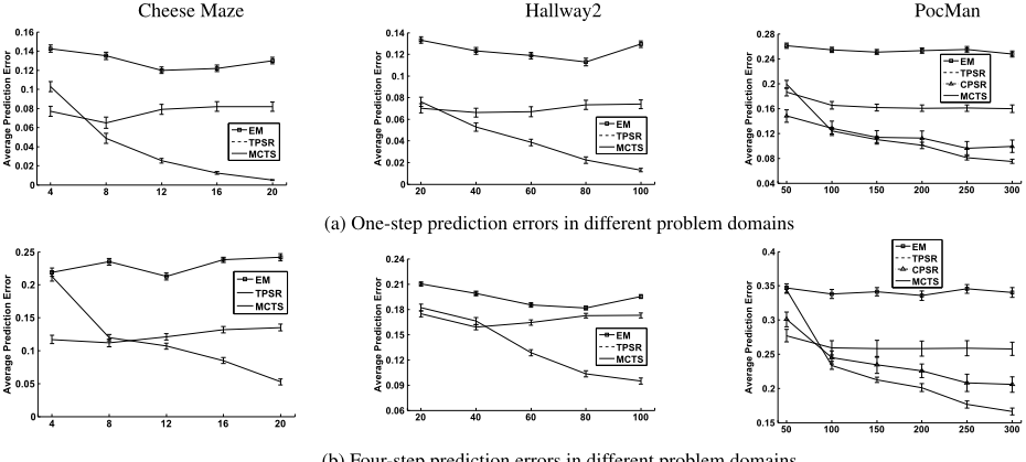
Fig. 1 compares the prediction accuracy of the evaluated methods in the three domains for one-step and four-step error respectively. In these figures, the x-axis is the number of nominal-states used for building the POMDP model (EM algorithm), the dimension of the representation used for representing state (TPSR/CPSR) or the number of discovered tests used for state representation, i.e., the search depth (Our approach, MCTS); the y-axis represents the mean error of the ten trials.

As can be seen from Fig. 1, both for the one-step and fourstep predictions, in almost all the cases, our algorithm performs very well and outperforms the other approaches. TPSR outperforms the EM algorithm. As the EM algorithm usually suffers from local minima, its performance is the poorest and the most unstable. For PocMan, although it is a domain suitable for the CPSR approach, compared to CPSR, our approach is still competitive. Considering the error reported is only the prediction error for one time step, the improvement on prediction accuracy on a long sequence is remarkable. Meanwhile, as the number of tests used for representing state increases, our algorithm reduces its prediction error while the other algorithms except for CPSR with increasing state number or dimension of the representation do not improve their performances and are unstable. We observe that in the lower dimension of the representation/number of tests, TPSR performs better than our method, however, in some cases, with increasing dimension of the representation, TPSR even performs worse. The intuitive explanation for this is that TPSR uses singular value decomposition (SVD) for dimension reduction, rather than just considering the information contained in the columns corresponding to the set of core tests, some information besides the set of core tests is also included in the obtained set of representation. When the dimension of the representation is far less than the number of the core tests, such information may be helpful; however, with the increase of the dimension of the representation, such information may add noise into the representation as we only need the information contained in the core tests.

5 RelatedWorks

In the PSRs literature, much attention has been devoted to learning PSR models. There are two main problems related to learn a PSR model [Rosencrantz et al., 2004]. One is the discovery problem, i.e., finding a small sufficient set of tests, called core tests, that can represent the state for the dynamical systems; the other is how to learn the model parameters to maintain a probability distribution over the discovered tests as the dynamical system progresses. As discussed in Technical Background section, once the set of core tests can be found, the model parameters can be learned easily.

According to the manner of how to address the discovery problem, there are two main approaches. One approach discovers the set of core tests using iterative methods. For linear PSRs, the vast majority of the literature on PSRs, one can derive the PSR model from a system dynamics matrix (SDM) that contains conditional probabilities of all possible tests given the past sequences [Singh and James, 2004]. The rank of the SDM is the linear dimension (denoted as k) of the dynamical system. The discovery problem is to find the tests corresponding to the k linearly independent columns of the SDM. As the number of tests in the SDM is infinite, the iterative approach works iteratively to obtain these tests. At each iteration, there is a current set ˆQ of core tests found so far, then the algorithm constructs two sub-SDMs, one sub-SDM's columns correspond to ˆQ, the other sub-SDM's columns correspond to ˆQ[ao ˆQ for each a 2 A and o 2 O. If the rank of these two sub-matrices equals to each other, ˆQ is used as the set of core tests. During the early stages of the PSRs research, almost all the work uses such iterative methods to discover the set of core test [James and Singh, 2004; Wolfe et al., 2005; Liu and Li, 2009; Liu et al., 2015]. However, such an approach is computation-expensive and time-consuming, also, the calculation of the rank of a noise matrix is usually not accurate and not stable, it is very difficult to find a satisfying set of core tests. This method is only applied to some toy problems with no more than dozen of states.

Recently, some work has been proposed to alleviate the discovery problem by specifying a large enough set of tests T so that it almost certainly contains a set of core tests [Boots et al., 2011; Boots and Gordon, 2011; Hamilton et al., 2013; 2014]. In these work, the discovery problem is avoided. The two main methods using such a strategy are transformed PSR (TPSR) and compressed PSR (CPSR). Currently, these two methods are also the most successful two learning methods for PSRs. For the TPSR approach [Boots et al., 2011; Boots and Gordon, 2011], to build the PSR model, one should estimate and manipulate two observable matrices PT↪H, PH,

(b) Four-step prediction errors in different problem domains

Figure 1: Prediction errors for difference cases in three problem domains.

and ♣A♣ ⇥ ♣O♣ observable matrices PT↪ao↪H. Although Denis et al. [Denis et al., 2014] showed that the concentration of the empirical PT↪H around its mean does not highly depend on its dimension, which gives a hope for alleviating the statistical problem when using large set of T and H as the accuracy of the learned model is directly connected to the concentration, manipulating these matrices is still too expensive to afford in large systems. At the same time, the TPSR approach requires singular value decomposition (SVD) on matrix PT↪H, for large set of T and H, such an operation is also prohibitively expensive. In our approach, instead of specifying and manipulating a large enough set of tests T in advance, we only use the found set of core tests (usually a very small subset of T) to estimate and manipulate the related matrices for building the PSR model, which is computationally cheap and more easy to manipulate.

By introducing a particular weighted loss function, Kulesza et al. [Kulesza et al., 2015a] proved that in the ideal setting where one can have access to the infinite SDM, compared to traditional spectral learning approaches, the performance of the learned TPSR model will be more stable and behave in a predictable way. They also demonstrated both theoretically and experimentally the importance of using large set of T and H when learning TPSR models. However, the statistic and computation issues are still not addressed.

To reduce the computational cost, rather than specifying a large enough set of tests, Kulesza et al. [Kulesza et al., 2015b] also tried to choose strategically a finite set of tests. However, there are important differences between their approach and ours, namely: (i) While our approach finds the core tests using MCTS directly, they first select a set of tests, then spectral method is applied by using these tests; (ii) MCTS can find the solution in a large space, while the work of [Kulesza et al., 2015b] just uses iterative approaches for selecting sets of tests, only a tiny part of the possible sets of tests can be considered; (iii) Most importantly, the key idea in [Kulesza et al., 2015b] is that as in the limiting-case, the singular values of the learned TPSR parameters are bounded, then under an assumption that smaller the singular values of the learned parameters are, more accuracy the learned TPSR model will be, they just select the tests that can cause smaller singular values of the learned TPSR parameters. However, no any formal guarantees are provided for such an approach.

Hamilton et al. [Hamilton et al., 2013; 2014] presented the CPSR model. This technique learns approximate PSR models by combining dimensionality reduction, incremental matrix decomposition, and compressed sensing. Compared to TPSR, CPSR allows for an increase in the efficiency and predictive power. However, different from our approach that has no prior assumptions on the environments to be modelled, CPSR can be only applied to domains with a particularly sparse structure.

6 Conclusion and FutureWork

In this paper, by utilizing the great merits of MCTS for finding solutions in large search spaces, a MCTS-based approach for discovering the set of core tests is presented, then the PSR model can be learned directly. In the process, the discovery problem is formalized as a sequential decision making problem and a concept of model entropy is proposed as the evaluation function of MCTS. Experimental results demonstrate the performance of our techniques. As also shown in the experiments, in order to accelerate the search process, we have focused our search on a limited search space by restricting the number of the legal actions at each node and the number of candidate actions, however, our methods still achieved significant performance compared to other approaches. With the expansion of the search space, we believe our method can achieve much better performance.

As MCTS requires computationally cheap reward to be computed in each iteration, in the future, we will focus our research on finding more efficient evaluation function for the discovery problem. Future work also includes verifying the effectiveness of our approach on more problems and planning with the learned PSR model.

Acknowledgments

This work was supported by the National Natural Science Foundation of China (No. 61375077 and 61375070). We would like to thank the anonymous reviewers for their valuable comments.