
Online Symbolic Gradient-Based Optimization for Factored Action MDPs
Proceedings of the Twenty-Fifth International Joint Conference on Artificial Intelligence. Pages 3075-3080.
© 2016 International Joint Conferences on Artificial Intelligence
Abstract
This paper investigates online stochastic planning for problems with large factored state and action spaces. We introduce a novel algorithm that builds a symbolic representation capturing an approximation of the action-value Q-function in terms of action variables, and then performs gradient based search to select an action for the current state. The algorithm can be seen as a symbolic extension of Monte-Carlo search, induced by independence assumptions on state and action variables, and augmented with gradients to speed up the search. This avoids the space explosion typically faced by symbolic methods, and the dearth of samples faced by Monte-Carlo methods when the action space is large. An experimental evaluation on benchmark problems shows that the algorithm is competitive with state of the art across problem sizes and that it provides significant improvements for large factored action spaces.
- [Barto et al., 1995] A. G. Barto, S. J. Bradtke, and A. P. Singh. Learning to act using real-time dynamic program- ming. Artificial Intelligence, 72:81-138, 1995.
- [Boutilier et al., 1995a] Craig Boutilier, Thomas Dean, and Steve Hanks. Planning under uncertainty: Structural as- sumptions and computational leverage. In Proceedings of the Second European Workshop on Planning, pages 157- 171, 1995.
- [Boutilier et al., 1995b] Craig Boutilier, Richard Dearden, Moises Goldszmidt, et al. Exploiting structure in policy construction. In Proc. of the International Joint Confer- ence on Artificial Intelligence, volume 14, pages 1104- 1113, 1995. IJCAI
- [Browne et al., 2012] Cameron B. Browne, Edward Pow- ley, Daniel Whitehouse, Simon M. Lucas, Peter I. Cowl- ing, Philipp Rohlfshagen, Stephen Tavener, Diego Perez, Spyridon Samothrakis, and Simon Colton. A survey of Monte Carlo tree search methods. Computational Intelli- gence and AI in Games, IEEE Transactions on, 4(1):1-43, 2012.
- [Cui et al., 2015] Hao Cui, Roni Khardon, Alan Fern, and Prasad Tadepalli. Factored MCTS for large scale stochas- tic planning. In Proc. of the AAAI Conference on Artificial Intelligence, 2015.
- [Domshlak and Hoffmann, 2006] Carmel Domshlak and Jörg Hoffmann. Fast probabilistic planning through weighted model counting. In Proc. of the International Conference on Automated Planning and Scheduling, pages 243-252, 2006.
- [Duchi et al., 2008] John C. Duchi, Shai Shalev-Shwartz, Yoram Singer, and Tushar Chandra. Efficient projec- tions onto the l 1 -ball for learning in high dimensions. In Proceedings of the International Conference on Machine Learning, pages 272-279, 2008.
- [Griewank and Walther, 2008] Andreas Griewank and An- drea Walther. Evaluating derivatives -principles and tech- niques of algorithmic differentiation (2. ed.). SIAM, 2008.
- [Hoey et al., 1999] Jesse Hoey, Robert St-Aubin, Alan Hu, and Craig Boutilier. SPUDD: Stochastic planning using decision diagrams. In Proceedings of the Workshop on Un- certainty in Artificial Intelligence, pages 279-288, 1999.
- [Keller and Helmert, 2013] Thomas Keller and Malte Helmert. Trial-based heuristic tree search for finite horizon MDPs. In Proc. of the International Conference on Automated Planning and Scheduling, 2013.
- [Kolobov et al., 2012] Andrey Kolobov, Peng Dai, Mausam Mausam, and Daniel S Weld. Reverse iterative deepening for finite-horizon MDPs with large branching factors. In Proc. of the International Conference on Automated Plan- ning and Scheduling, 2012.
- [Lang and Toussaint, 2010] Tobias Lang and Marc Tous- saint. Planning with noisy probabilistic relational rules. Journal of Artificial Intelligence Research, 39:1-49, 2010.
- [Lee et al., 2014] Junkyu Lee, Radu Marinescu, and Rina Dechter. Applying marginal MAP search to probabilistic conformant planning: Initial results. In AAAI Workshop on Statistical Relational Artificial Intelligence, 2014.
- [Murphy and Weiss, 2001] Kevin Murphy and Yair Weiss. The factored frontier algorithm for approximate inference in DBNs. In Proceedings of the Workshop on Uncertainty in Artificial Intelligence, pages 378-385, 2001.
- [Palacios and Geffner, 2009] Héctor Palacios and Hector Geffner. Compiling uncertainty away in conformant plan- ning problems with bounded width. Journal of Artificial Intelligence Research (JAIR), 35:623-675, 2009.
- [M. L. Puterman. Markov decision pro- cesses: Discrete stochastic dynamic programming. Wiley, 1994. Raghavan et al., 2012] Aswin Raghavan, Saket Joshi, Alan Fern, Prasad Tadepalli, and Roni Khardon. Planning in factored action spaces with symbolic dynamic program- ming. In Proc. of the AAAI Conference on Artificial Intel- ligence, 2012.
- [Raghavan et al., 2013] Aswin Raghavan, Roni Khardon, Alan Fern, and Prasad Tadepalli. Symbolic opportunis- tic policy iteration for factored-action MDPs. In Advances in Neural Information Processing Systems, pages 2499- 2507, 2013.
- [Sang et al., 2005] Tian Sang, Paul Beame, and Henry A. Kautz. Performing bayesian inference by weighted model counting. In Proc. of the National Conference on Artificial Intelligence, pages 475-482, 2005.
- [Sanner, 2010] Scott Sanner. Relational dynamic influ- ence diagram language (RDDL): Language description. Unpublished Manuscript. Australian National University, 2010.
- [Shalev-Shwartz, 2012] Shai Shalev-Shwartz. Online learn- ing and online convex optimization. Foundations and Trends in Machine Learning, 4(2):107-194, 2012.
- [Tesauro and Galperin, 1996] Gerald Tesauro and Gregory R Galperin. On-line policy improvement using monte-carlo search. In Advances in Neural Information Processing Sys- tems, pages 1068-1074, 1996.
- [Tesauro, 1992] G. Tesauro. Temporal difference learning of backgammon strategy. In Proceedings of the International Conference on Machine Learning, pages 451-457, 1992.
- [Wainwright and Jordan, 2008] Martin J. Wainwright and Michael I. Jordan. Graphical models, exponential fami- lies, and variational inference. Foundations and Trends R in Machine Learning, 1(1-2):1-305, 2008.
- [Wang and Carreira-Perpiñán, 2013] Weiran Wang and Miguel Á. Carreira-Perpiñán. Projection onto the proba- bility simplex: An efficient algorithm with a simple proof, and an application. CoRR/arXiv, abs/1309.1541, 2013.
- [Williams, 1992] Ronald J. Williams. Simple statistical gradient-following algorithms for connectionist reinforce- ment learning. Machine Learning, pages 229-256, 1992.
References were extracted automatically from the PDF and may contain errors.
Full text extracted automatically from the PDF; figures, tables and equations may differ. The PDF is the version of record.
1 Introduction
Recently there is increased interest in stochastic planning in domains with large combinatorially structured action spaces. Such structure arises, for example, when multiple units can operate in parallel to achieve a joint objective. Such problems have been modeled using factored Markov decision processes (MDP) where state and action descriptions are composed of the values of sets of variables. Factored MDPs have been investigated with a variety of approaches which are reviewed in the next section including symbolic dynamic programming, probabilistic inference, Monte Carlo Search, linear function approximation and more. However, apart from function approximation with manually tuned representations, scalability to large action spaces is still a significant challenge. Notably, methods that rely on exact representation of value functions are space bound due to the inherent complexity of representing the corresponding functions. On the other hand symbolic search based methods are not able to explore the space sufficiently when given a strict time limit for action selection.
The main contribution of this paper is a novel algorithm that offers such scalability. The algorithm is based on the idea of Monte Carlo search with a strong simplifying assumption on independence of state and action variables. Such assumptions are common in variational inference [Wainwright and Jordan, 2008], and have been used for estimation in state space models [Murphy and Weiss, 2001] and even for planning [Lang and Toussaint, 2010]. Our recent work [Cui et al., 2015] made the observation that, under this assumption, sampling of trajectories can be done in aggregate form by rewriting the transition model as algebraic expressions and then computing marginals on state variables by direct calculation instead of explicit sampling. While this efficiently samples trajectories for a given root action it requires action enumeration and does not scale for large action spaces.
In this paper we make two additional observations. First, the algebraic computation can be done symbolically. We show how the sampled trajectories and the corresponding marginals can be captured using an explicit graph representing the computation, where the state marginals and the reward are functions of action variables. Second, given this graph, we can calculate gradients and perform gradient ascent over the action space, effectively optimizing the action for the current state. Several additional algorithmic ideas make for a robust search algorithm that dynamically adjusts to the problem and balances the benefits of Monte Carlo search and gradients. An extensive experimental evaluation demonstrates that the algorithm performs significantly better than previous work and that all its components contribute to that success.
2 Background and RelatedWork
This section gives a brief review of factored MDPs and related algorithms. A MDP [Puterman, 1994] is specified by ¶S↪A↪ T↪R↪ γ♦, where S is a finite state space, A is a finite action space, T(s↪ a↪ s0 ) = p(s0 ♣s↪ a) defines the transition probabilities, R(s↪ a) is the immediate reward of taking action a in state s, and γ is the discount factor. A policy ⇡ : S ! A is a mapping from states to actions, indicating which action to choose at each state. Given a policy ⇡, the value function V ⇡ (s) is the expected discounted total reward E[Pi γ iR(si↪ ⇡(si)) ♣ ⇡], where si is the ith state visited by following ⇡ (and s0 = s). The action-value function Q⇡ : S ⇥ A ! R is the expected discounted total reward when taking action a at state s and following ⇡ thereafter.
MDPs with large state and action spaces are typically represented in factored form [Boutilier et al., 1995a]. The state space S is specified by a set of binary variables ¶x1↪ ▷ ▷ ▷ ↪ xl♦ so that ♣S♣ = 2l . Similarly, A is specified by a set of binary variables ¶y1↪ ▷ ▷ ▷ ↪ ym♦ so that ♣A♣ = 2m. Often, when domains are described using a higher level language, action constraints limit the choice of legal actions so that ♣A♣ < 2m.
Basic MDP optimization algorithms require enumeration over states and actions making them impractical for large problems. Symbolic versions of these algorithms have been developed for factored state and action spaces [Hoey et al., 1999; Boutilier et al., 1995b; Raghavan et al., 2012; 2013]. However, scalability is still problematic due to the description size of value functions and policies. Parametric methods represent the value function using some compact representation (e.g., as a linear function over a fixed feature space) and thus avoid the space problem. Such approaches have been very successful in reinforcement learning [Tesauro, 1992] and in policy gradient algorithms [Williams, 1992].
Online planning avoids the space complexity by focusing on choosing a high-quality action for the current state and repeatedly applying this procedure to states visited. The Rollout Algorithm [Tesauro and Galperin, 1996], which performs one step lookahead from the current state, is the simplest such procedure. In particular, given a state s and baseline policy ⇡, the rollout algorithm calculates an estimate of Q⇡ (s↪ a) for each action a and then picks the a maximizing this value. To estimate Q⇡ (s↪ a) simply use the MDP model to sample s0 from p(s0 ♣s↪ a) and then apply ⇡ for h steps where h is the desired horizon. Repeating this and averaging we get an estimate for Q⇡ (s↪ a). More sophisticated online planning methods include real time dynamic programming [Barto et al., 1995] and Monte Carlo Tree Search (MCTS) [Browne et al., 2012] and the Gourmand [Kolobov et al., 2012] and PROST [Keller and Helmert, 2013] systems based on these have won top places in recent planning competitions.
The performance of sample based Rollout procedures degrades significantly when the action space is large because one has to sample multiple trajectories for each action in order to get reasonable estimates. With combinatorial action spaces there are very few samples per action and the estimates have high variance and are not reliable. The ARollout algorithm [Cui et al., 2015] is a heuristic that attempts to address this issue. Since our algorithm uses some of the ideas from ARollout we describe it in more detail in the next section.
2.1 The ARollout Algorithm
We illustrate the ARollout algorithm using the following example. In this example, as in our implementation, we use the RDDL language [Sanner, 2010] to specify the domain. The problem has three state variables s(1), s(2) and s(3), and three action variables a(1), a(2), a(3) respectively. In addition we have two intermediate variables cond1 and cond2 which are not part of the state. The dynamics is given by the following expressions where primed variants of variables represent the value of the variable after performing the action.
cond1 = Bernoulli(0.7) cond2 = Bernoulli(0.5) s'(1) = if (cond1) then ˜a(3) else false s'(2) = if (s(1)) then a(2) else false s'(3) = if (cond2) then s(2) else false reward = s(1) + s(2) + s(3)ARollout translates the RDDL code into algebraic expressions using standard transformations from a logical to a numerical representation. In our example this yields:
s'(1) = (1-a(3))*0.7 s'(2) = s(1)*a(2) s'(3) = s(2)/2 r = s(1) + s(2) + s(3)These expressions are used for efficient approximation of marginal distributions over state variables, and the distribution is used to estimate the Q function. Like Rollout, to estimate Q⇡ (s↪ a) ARollout first samples s0 from p(s0 ♣s↪ a). However, unlike Rollout, instead of simulating individual trajectories, ARollout approximates the simulation of state distributions through their marginals over individual variables.
To illustrate, let the sampled s0 be s0 = ¶s(1)=1↪ s(2)= 1↪ s(3)=1♦. ARollout first translates s0 into a representation of marginals over individual variables, referred to as aggregate states and denoted as. In this case, as0 = ¶s(1)=1↪ s(2)=1↪ s(3)=1♦. The algorithm then calculates marginals over action variables which are induced by using the rollout policy ⇡ in the current aggregate state as. This can be estimated by first sampling a concrete state cs from as, then calculating the action ca = ⇡(cs) and averaging over action variable values. For our example, assume that this yields aa0 = ¶a(1)=0▷3↪ a(2)=0▷4↪ a(3)=0▷3♦. The reward r0 from the current state and action is estimated by directly plugging in the values of each variable into the expression for r. So we get r0 = 1 + 1 + 1 = 3. Similarly, as1 is obtained by substituting marginals into the expressions for state variables. In this case, as1 = ¶s0 (1)=(1 - 0▷3) ⇤ 0▷7=0▷49↪ s0 (2)=1 ⇤ 0▷4=0▷4↪ s0 (3)=0▷5♦. The algorithm continues in this manner, computing aggregate actions, aggregate states and estimating the reward to the required depth. This provides one aggregate trajectory. This simulation is correct under extreme assumptions [Cui et al., 2015] and it can be seen as a heuristic estimate when the conditions do not hold.
ARollout repeats this to obtain multiple aggregate trajectories per action and averages the reward to get Q⇡ (s↪ a). This process is repeated for every action a, and the maximizing a is picked to be used in the current state. ARollout's estimates are more stable than Rollout's estimates but the need to enumerate actions limits applicability to large action space.
3 Gradient Based Optimization
The main contribution of this paper is to provide an algorithm that scales successfully for factored action spaces. The algorithm is based on two important observations. The first is that the calculation illustrated in the previous section can be performed symbolically to yield a compact expression capturing the approximation of the Q function as a function of action variables. The second is that, once such a representation exists, one can use gradient based optimization to search for the best action in the current state. Several additional ideas are used to make the search more robust and to diversify its exploration. We denote this algorithm as SOGBOFA (symbolic online gradient based optimization for factored actions).
The input to SOGBOFA is the same as in ARollout. As explained below, we assume that constraints over legal actions, if they exist, are given as sum constraints (sum of all or some variables is bounded, e.g., concurrency constraints). Unlike ARollout, SOGBOFA maintains an aggregate action aa for the current state. This represents a distribution over actions to be chosen in the current state. The algorithm is as follows:
SOGBOFA(S)
1 Qf BuildQf(S↪ timeAllowed) 2 As = ¶ ♦ 3 while time remaining 4 do A RandomRestart() 5 while time remaining and not converged 6 do D CalculateGradient(Qf) 7 A MakeUpdates(D) 8 A Projection(A) 9 As▷add(SampleConcreteAct(A)) 10 action Best(As)Overview of the Algorihm: In line 1, we build an expression graph that represents the approximation of the Q function. This step also explicitly optimizes a tradeoff between simulation depth and run time to ensure that enough updates can be made. Line 4 samples an initial action for the gradient search. Lines 6 to 8 calculate the gradient and make an update on the aggregate action. Line 9 makes the search more robust by finding a concrete action induced by the current aggregate action and evaluating it explicitly. Line 10 picks the action with the maximum estimate. Line 5 checks our stopping criterion which allows us to balance gradient and random exploration. In the following we describe these steps in more details.
Building a symbolic representation of the Q function: We build a DAG representing the Q function by expanding from the current state one level at a time. The depth of this process, which is equivalent to the search depth in standard algorithms, is determined dynamically as explained below. The construction is analogous to the construction of expression trees in a compiler. Leaf nodes represent either constants or state or action variables. Internal nodes represent algebraic operations over the children. Our implementation uses +↪-↪ ⇤↪ ◁ as operations but it can be easily extended to include other operations. The implementation directly follows the algebraic expressions compiled from the RDDL description (as in ARollout) to build explicit expression DAGs. The only exception is the flattening of multiple levels of + or ⇤; for example (+(+(a↪ b))↪ c) is flattened to +(a↪ b↪ c).
We start from representing each initial state variable as a leaf node whose value is 0 or 1. We also represent each action variable at the initial state as a leaf node. In this case the node represents the marginal probability of that variable, serving as a parameter to be optimized. For each step of expansion, we create a copy of the algebraic expressions in DAG form. To simulate the rollout, action variables other than at the root are given a numerical value capturing the marginal probability over the action variable induced by ⇡. The marginals can be calculated dynamically exactly as in ARollout. In the experiments in this paper we report on rollout of the random policy where marginals can be calculated explicitly even with sum constraints. 1 If the MDP domain requires discounting we add this to the expression tree. The sum of discounted rewards is the estimate of the Q value. Figure 1 illustrates the construction for our example for horizon 1. For deeper horizons this construction is repeated sequentially.
1 For example, if the constraints choose at most k bits out of n to
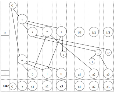
We note that action variables at levels 2 and above (nodes with value 1/3 in the figure) can also be treated as parameters, exactly as the variables of the first level. This leads to an algorithm related to conformant planning. We discuss this idea further in the concluding section of the paper.
Dynamic control over simulation depth: In principle we should build the DAG to the horizon depth. However, if the DAG is large then evaluation of Q⇡ (s↪ a) and gradient computation are expensive so that the number of actions explored in the search might be too small. This tradeoff must be controlled by any domain independent online search algorithm.
Our algorithm limits depth when the expected number of gradient updates is below a pre-fixed threshold. This can be done dynamically. In particular we estimate if the time left is sufficient for building one more level of the DAG and making enough updates. The time cost of adding one level to the DAG, ta, is independent of the level and can be estimated by the average of the previous levels. The time cost of an update at the current level, tI, is estimated by simulated updates on the current DAG (we use min¶0▷3 ⇤ NumberOfLegalAction↪ 5♦ updates). We estimate tI+1, by tI +∆t where ∆t is the average increase in cost over previous levels. Finally, we expand one more level if ta+k⇤tI+1 is smaller than the remaining time, guaranteeing at least k expected updates (where k = 200 in our experiments).
Random Restarts: A random restart generates a concrete (binary) legal action in the state.
Calculating the gradient: The main observation is that once the graph is built, representing Q as a function of action variables, we can calculate gradients using the method of automatic differentiation [Griewank and Walther, 2008]. This is a
standard method that has also been recently used in machine learning. Our implementation uses the reverse accumulation method since it is more efficient having linear complexity in the size of the DAG for calculation of all gradients. Intuitively, the idea can be seen to generalize the backpropagation algorithm for learning in neural networks to an arbitrary computational circuit. Since the ideas are well known we refer the reader to [Griewank and Walther, 2008] for details.
Maintaining action constraints: Gradient updates allow the values of marginal probabilities to violate the [0↪ 1] constraints as well as constraints on legal actions. To handle this issue we use a standard algorithm, projected gradient ascent [Shalev-Shwartz, 2012], where one first takes a gradient step and then projects the values back to the legal region.
Projection onto combinatorial constraints can be computationally expensive. Our implementation limits allowed constraints to sum constraints over action variables. This is typical, for example, in high level representations that use 1-ofk representation for actions where at most one bit among a group of k should be set to 1. It is important to enforce these constraints during search. If this is not done then, if all actions are somewhat useful, we will end up with the uninformative choice of setting all variables to 1.
Our algorithm supports multiple sum constraints. As a first step we clip all values to the [0↪ 1] range. We then iteratively project to respect all sum constraints. To achieve this we use a known algorithm [Wang and Carreira-Perpi˜n´an, 2013; Duchi et al., 2008] to project onto a scaled probability simplex P ai B for a given bound B. The algorithm repeatedly subtracts the surplus amount from all non-zero entries, clipping at 0. For example, given ¶1▷2↪ 1↪ 0▷9↪ 0▷5↪ 0▷1♦ and B = 2, we subtract (3▷7 - 2)◁5 = 0▷34 from each entry (clipping the last) to get ¶0▷86↪ 0▷66↪ 0▷56↪ 0▷16↪ 0♦ and then subtract 0▷24◁4 = 0▷06 to get ¶0▷8↪ 0▷6↪ 0▷5↪ 0▷1↪ 0♦.
Optimizing step size for gradient update: Gradient ascent often works well with a constant step size. However, in some problems, when the rollout policy is random, the effect of the first action on Q is very small implying that the gradient is very small and a fixed step size is not suitable. We therefore search for an appropriate step size. To mitigate the fact that we are using continuous search over the discrete space we use a brute force search instead of standard line search.
We first choose a range for ↵ with enough flexibility so that any ↵ 2 [0↪ maxAlpha] won't push the variables beyond maxV ar + 1 or below -1 where maxV ar is the max value among the variables. We then perform a linear search using 10 evenly spaced values a0↪ a1▷▷▷a9 in that region to find the best ↵ where quality is measured by the value of the Q function DAG. If the best ↵ happens to be a0, implying that the original maxAlpha may not be at the right scale, we reset the legal region to be [0↪ a0] and run the process again. This is repeated until the best ↵ is not a0 with a max of 5 levels.
Sampling concrete Actions: The gradient optimization performs a continuous search over the discrete space. This means that the values given by the Q are not always reliable on the fractional aggregate actions. To add robustness we associate each aggregate action encountered in the search with a concrete action chosen from its distribution and record the more reliable value of the concrete action. Search proceeds as usual with the aggregate actions but final action selection is done using these more reliable scores for concrete actions.
Selecting a concrete action from the aggregate one can be formulated as a weighted max SAT problem similar to [Sang et al., 2005]. However, this is an expensive calculation. We therefore use a heuristic that picks action variables with highest marginal probabilities as follows. We first sort action variables by their marginal probabilities. We then add active action bits as long as the marginal probability is not lower than marginal probability of random rollout and the constraints are not violated. For example, suppose the marginals are ¶0▷8↪ 0▷6↪ 0▷5↪ 0▷1↪ 0♦, B = 3, and we use a threshold of 0▷55. Then we have ¶a1↪ a2♦ as the final action.
Stopping Criterion: Our results show that gradient information is useful. However, getting precise values for the marginals at local optima is not needed, because small changes are not likely to affect the choice of concrete action. We thus use a loose criterion aiming to allow for a few gradient steps but to quit relatively early so as to allow for multiple restarts. Our implementation stops the gradient search if the max change in probability is less than S = 0▷1, that is, kAnew - Aoldk1 0▷1. The result is an algorithm that combines Monte Carlo search and gradient based search.
4 Experimental Evaluation
We evaluate the SOGBOFA algorithm on several domains showing its advantage and in addition present an ablation study that shows that different components of the algorithm contribute to this success. The evaluation is done over 6 domains, elevators from the RDDL distribution, two from the International Probabilistic Planning Competition (IPPC) 2011, and three from IPPC 2014 where we chose domains amenable to expansion of the action space. We follow the setting of [Cui et al., 2015] and use the 10 competition problems (index 1 to 10) but add 10 more challenging instances in each domain (index 11 to 20). The size of the action space in these problems is shown in Table 1. The reported results represent averages from 20 runs in each problem instance where each instance is run for 40 time steps. In these runs each algorithm is given 60 seconds per step (on a cluster node having Intel Xeon X5675@ 3GHz CPU, and 24GB memory).
As baselines we compare against Rollout and MCTS that work by sampling concrete trajectories and against ARollout. As in [Cui et al., 2015], these algorithms simulate trajectories for min¶20↪ horizon♦ steps, which we denote as HalfDepth below. The work of [Cui et al., 2015] showed that on large factored spaces ARollout dominates PROST [Keller and Helmert, 2013] the winner of the recent IPPC so the comparison to ARollout serves as a reference point to state of the art. For visual clarity we rescale reward values relative to the values achieved by the random policy (as zero) and the value achieved by a simple hand coded policy for the domain (as 1) or against the value of one of the algorithms (which is the reference value of 1 in that case).
In addition we test several variants of the algorithm with some of the features disabled to investigate their contribution. In particular SARollout (Symbolic ARollout) uses the DAG
| Problem | 6 | 7 | 8 | 9 | 10 | 11 | 12 | 13 | 14 | 15 | 16 | 17 | 18 | 19 | 20 |
| elevators | 16 | 64 | 64 | 64 | 256 | 256 | 256 | 1024 | 1024 | 1024 | 4096 | 4096 | 4096 | 16384 | 16384 |
| sysadmin | 31 | 41 | 41 | 51 | 51 | 3241 | 5051 | 7261 | 366276 | 562626 | 682801 | 972151 | 5.3E7 | 6.6E7 | 2.6E9 |
| traffic | 16 | 16 | 16 | 16 | 16 | 512 | 512 | 512 | 4096 | 4096 | 4096 | 65536 | 65536 | 65536 | 65536 |
| skill | 13 | 15 | 15 | 17 | 17 | 211 | 6580 | 52956 | 974982 | 1.8E7 | 5.6E8 | 8.5E9 | 2.6E11 | 5.1E12 | 4.8E13 |
| academic | 211 | 26 | 326 | 31 | 466 | 12384 | 231526 | 4216423 | 1.7E8 | 3.5E9 | 1.9E11 | 4.2E12 | 9.9E13 | 3.1E15 | 1.9E17 |
| tamarisk | 13 | 15 | 15 | 17 | 17 | 172 | 1351 | 12951 | 122438 | 1149017 | 1.0E7 | 1.0E8 | 9.3E8 | 8.6E9 | 8.0E10 |
construction but does not use gradients at all. This algorithm is identical to ARollout in terms of its individual estimates but it provides speedup because the DAG is reused across samples. Comparing against SARollout allows us to separate the contribution of the symbolic computation from the gradients. We also use variants with dynamic depth disabled, and with the dynamic setting of step size disabled, illustrate the contribution of the projection step, and show both the importance of the stopping criterion and insensitivity to its precise setting.
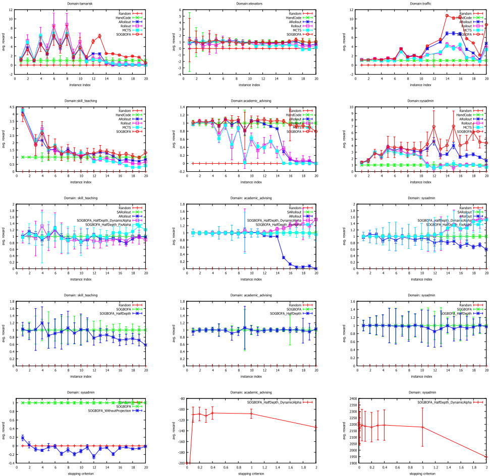
The top two rows in Figure 2 show a comparison of SOGBOFA to the baselines in all 6 domains showing a significant advantage on the problems with large action spaces.
The third row of Figure 2 shows a comparison to SARollout where for clarity in the comparison SARollout uses HalfDepth, exactly as Rollout. In addition these plots compare to HalfDepth variants of the gradient based algorithm with fixed ↵ = 0▷1 vs. the dynamic setting. Due to space constraints we only show results for 3 of the domains but the other 3 domains show similar behavior. The plots show that SARollout dominates ARollout thus illustrating the significance of the symbolic representation even without gradients. They also show that the gradient based algorithms with HalfDepth either dominate SARollout or are comparable.
The choice between fixed and dynamic ↵ represents a tradeoff. They mostly perform pretty closely but in some cases one of the two dominates significantly. The importance of the dynamic selection of ↵ arises in some of the large problems (e.g., academic advising 16-20) where the gradient with respect to action variables is very small (around -1E-16 ), and fixing the alpha to a small value makes for tiny updates that make no progress. We prefer the dynamic setting as it can adapt to the shape of the Q function more robustly.
It is insightful to look at the number of concrete actions seen by SARollout and the gradient algorithms. When inspected (details omitted) we observe that SARollout sees many more actions, in some cases more than 10 fold more, than the dynamic ↵ variant. Nonetheless, the gradient algorithms that see less actions have better performance.
The fourth row of Figure 2 evaluates the contribution of dynamic depth selection for 3 domains. Results for the other domains are omitted due to space constraints and they show similar trends. We can observe that dynamic depth is comparable and in some cases significantly better than fixed depth.
The left plot in the fifth row of Figure 2 illustrates that projection is crucial on the sysadmin domain. In this case, without projection the algorithm is not distinguishable from the random policy. The remaining plots in the fifth row illustrate the importance of the tradeoff given by the stopping criterion. Results are shown as a function of the L1 bound S (S=0▷1 in the main algorithm). The plots show results for S in the range
10-9 (very strict criterion, few restarts) to 1 (always stop after one gradient update) for problem 20 of sysadmin and academic advising. For reference we also include the SARollout algorithm which makes no updates, and this is represented in the plot at the point S = 2. The results show that neither extreme is a good choice, that a criterion balancing gradients and Monte Carlo steps provides better performance and that there is a large range of values that provide this tradeoff.
5 Conclusion
The paper presented a novel algorithm for stochastic planning in factored spaces that scales well to very large action spaces. The main idea is to use symbolic simulation with an explicit approximation induced by independence assumptions, and to perform gradient search to maximize the Q function using this symbolic representation. Several algorithmic tools serve to make the algorithm robust, including dynamic choice of simulation depth, dynamic choice of gradient step size, shadowing the gradient search with a search over concrete actions, and a balance between gradients and random restarts. The experiments demonstrate that the algorithm is significantly better than previous work and that the different components of the algorithm contribute to that success.
The algorithm also suggests an intriguing opportunity going beyond symbolic rollouts. In particular, as described above, when constructing the DAG we can leave all action variables in their symbolic form. In that case the Q function is a function of all action variables in all time steps. Selecting concrete values for all these variables is the same as deciding on the entire sequence of actions in advance of execution. This is known as conformant planning [Palacios and Geffner, 2009; Domshlak and Hoffmann, 2006; Lee et al., 2014]. Interestingly, reverse accumulation automatic differentiation allows us to perform gradient steps over all these variables without an increase in run time. We can therefore use essentially the same method to optimize an approximation of conformant planning. This has the potential to improve over SOGBOFA, especially when rolling out the random policy is not informative. Preliminary experiments suggest that such improvement is obtained in some cases but that in many cases the large scale optimization leads to degradation in performance. We leave exploration of this optimization challenge for future work.
Acknowledgments
We are grateful to Alan Fern, Prasad Tadepalli and Scott Sanner for helpful discussions. This work was partly supported by NSF under grant IIS-0964457. Some of the experiments in this paper were performed on the Tufts Linux Research Cluster supported by Tufts Technology Services.
@inproceedings{ijcai2016p436,
  title     = {Online Symbolic Gradient-Based Optimization for Factored Action MDPs},
  author    = {Cui, Hao and Khardon, Roni},
  booktitle = {Proceedings of the Twenty-Fifth International Joint Conference on
               Artificial Intelligence, {IJCAI-16}},
  publisher = {AAAI Press / International Joint Conferences on Artificial Intelligence},
  editor    = {Subbarao Kambhampati},
  pages     = {3075--3080},
  year      = {2016},
  month     = {7},
  url       = {https://ijcai.org/proceedings/2016/436},
}
TY - CPAPER TI - Online Symbolic Gradient-Based Optimization for Factored Action MDPs AU - Cui, Hao AU - Khardon, Roni T2 - Proceedings of the Twenty-Fifth International Joint Conference on Artificial Intelligence, IJCAI-16 PB - AAAI Press / International Joint Conferences on Artificial Intelligence PY - 2016 SP - 3075 EP - 3080 UR - https://ijcai.org/proceedings/2016/436 ER -Copied
Machine-readable versions of this paper, for tools and AI agents:





