
Stochastic Multiresolution Persistent Homology Kernel
Proceedings of the Twenty-Fifth International Joint Conference on Artificial Intelligence. Pages 2449-2456.
© 2016 International Joint Conferences on Artificial Intelligence
Abstract
We introduce a new topological feature representation for point cloud objects. Specifically, we construct a Stochastic Multiresolution Persistent Homology (SMURPH) kernel which represents an object's persistent homology at different resolutions. Under the SMURPH kernel two objects are similar if they have similar number and sizes of holes at these resolutions. Our multiresolution kernel can capture both global topology and fine-grained topological texture in the data. Importantly, on large point clouds the SMURPH kernel is more computationally tractable compared to existing topological data analysis methods. We demonstrate SMURPH's potential for clustering and classification on several applications, including eye disease classification and human activity recognition.
- [Ahmed et al., 2014] Mahmuda Ahmed, Brittany Terese Fasy, and Carola Wenk. Local persistent homology based distance between maps. In SIGSPATIAL. ACM, Nov. 2014.
- [Altun et al., 2010] Kerem Altun, Billur Barshan, and Orkun Tuncel. Comparative study on classifying human activi- ties with miniature inertial and magnetic sensors. Pattern Recognition, 43(10):3605 -3620, 2010.
- [Bubenik, 2015] Peter Bubenik. Statistical topological data analysis using persistence landscapes. Journal of Machine Learning Research, 16:77-102, 2015.
- [Carlsson, 2009] Gunnar Carlsson. Topology and data. Bul- letin (New Series) of the American Mathematical Society, 46(2):255-308, 2009.
- [Chazal et al., 2013] F. Chazal, B. T. Fasy, F. Lecci, A. Ri- naldo, A. Singh, and L. Wasserman. On the Bootstrap for Persistence Diagrams and Landscapes. arXiv preprint arXiv:1311.0376, November 2013.
- [Chazal et al., 2015a] F. Chazal, B. T. Fasy, F. Lecci, B. Michel, A. Rinaldo, and L. Wasserman. Subsampling Methods for Persistent Homology. In ICML15, 32nd Inter- national Conference on Machine Learning, Lille, France, 2015.
- [Chazal et al., 2015b] Frédéric Chazal, Brittany Terese Fasy, Fabrizio Lecci, Alessandro Rinaldo, and Larry A. Wasser- man. Stochastic convergence of persistence landscapes and silhouettes. Journal of Computational Geometry, 2015. To appear.
- [Edelsbrunner and Harer, 2010] H. Edelsbrunner and J. Harer. Computational Topology: An Introduction. Applied mathematics. Amer Mathematical Society, 2010.
- [Fasy et al., 2014] Brittany T. Fasy, Jisu Kim, Fabrizio Lecci, and Clement Maria. TDA: Statistical tools for topological data analysis. http://cran.r-project.org/web/ packages/TDA, 2014. Link
- [Hoover and Goldbaum, 2013] Adam Hoover and Michael Goldbaum. Stare public onine database, 2013. http: //www.ces.clemson.edu/ ⇠ ahoover/stare/. Link
- [Joachims, 2008] Thorsten Joachims. SVM light support vec- tor machine, 2008. http://svmlight.joachims.org/. Link
- [Karatzoglou et al., 2004] Alexandros Karatzoglou, Alex Smola, Kurt Hornik, and Achim Zeileis. kernlab -an S4 package for kernel methods in R. Journal of Statistical Software, 11(9):1-20, 2004.
- [Kwitt et al., 2015] Roland Kwitt, Stefan Huber, Marc Ni- ethammer, Weili Lin, and Ulrich Bauer. Statistical topo- logical data analysis -a kernel perspective. In C. Cortes, N.D. Lawrence, D.D. Lee, M. Sugiyama, and R. Garnett, editors, Advances in Neural Information Processing Sys- tems 28, pages 3052-3060.
- Curran Associates, Inc., 2015.
- [Li et al., 2014] Chunyuan Li, Maks Ovsjanikov, and Fred- eric Chazal. Persistence-based structural recognition. The IEEE Conference on Computer Vision and Pattern Recog- nition (CVPR), June 2014.
- [Maria, 2014] C. Maria. Gudhi, simplicial complexes and persistent homology packages. https://project.inria.fr/ gudhi/software/, 2014. Link
- [Morozov, 2007] Dmitriy Morozov. Dionysus, a c++ library for computing persistent homology. http://www.mrzv.org/ software/dionysus/, 2007. Link
- [Nanda and Sazdanović, 2014] Vidit Nanda and Radmila Sazdanović. Simplicial models and topological inference in biological systems. In Natasa Jonoska and Masahico Saito, editors, Discrete and Topological Models in Molec- ular Biology. Springer, 2014.
- [Nanda, 2013] Vidit Nanda. Perseus, the persistent ho- mology software. http://www.sas.upenn.edu/ ⇠ vnanda/ perseus, 2013. Accessed Aug. 6, 2014. Link
- [Neumann et al., 2013] M. Neumann, P. Moreno, L. An- tanas, R. Garnett, and K. Kersting. Graph Kernels for Ob- ject Category Prediction in Task-Dependent Robot Grasp- ing. In Proceedings of the Eleventh Workshop on Min- ing and Learning with Graphs (MLG-2013), Chicago, US, 2013.
- [Pachauri et al., 2011] Deepti Pachauri, Chris Hinrichs, Moo K. Chung, Sterling C. Johnson, and Vikas Singh. Topology-based kernels with application to inference problems in alzheimer's disease. IEEE Trans. Med. Imag- ing, 30(10):1760-1770, 2011.
- [Reininghaus et al., 2015] Jan Reininghaus, Stefan Huber, Ulrich Bauer, and Roland Kwitt. A stable multi-scale kernel for topological machine learning. The IEEE Con- ference on Computer Vision and Pattern Recognition (CVPR), 2015.
- [Tausz et al., 2011] Andrew Tausz, Mikael Vejdemo- Johansson, and Henry Adams. Javaplex: A research software package for persistent (co)homology. Software available at http://appliedtopology.github.io/javaplex/, 2011. Link
- [Zhu, 2013] Xiaojin Zhu. Persistent homology: An intro- duction and a new text representation for natural language processing. In The 23rd International Joint Conference on Artificial Intelligence (IJCAI), 2013. IJCAI
References were extracted automatically from the PDF and may contain errors.
Full text extracted automatically from the PDF; figures, tables and equations may differ. The PDF is the version of record.
1 Introduction and Background
There has been growing interest in bringing topological data analysis (TDA) into machine learning [Bubenik, 2015; Chazal et al., 2015b; Reininghaus et al., 2015; Ahmed et al., 2014; Li et al., 2014; Chazal et al., 2015a; Pachauri et al., 2011]. However, no method exists that is simultaneously rich in topological information, efficient in computation, and easy to plug into a machine learning system. We take a step in this direction by proposing a Stochastic MUltiResolution Persistent Homology (SMURPH) kernel. Our kernel can be viewed as a topological feature extractor for machine learning that compares the number and sizes of "holes" in two point clouds. Unlike prior TDA methods, SMURPH captures both the global topology and fine-grained "topological texture" in point cloud objects. Using SMURPH for machine learning requires little background in topology, as it just produces a kernel matrix.
Persistent homology is a TDA method for studying homology classes, or "topological holes." A thorough tutorial is out of scope of this paper and can be found in e.g. [Edelsbrunner and Harer, 2010; Nanda and Sazdanovi´c, 2014; Carlsson, 2009; Zhu, 2013]. We will focus on first-order homology over Z2 (binary) coefficients. For this purpose the following background knowledge suffices. On a point cloud X in Rd we construct an ✏-hypergraph by creating edges
(known as 1-simplices) between all pair of points xi↪ xj 2 X within distance ✏. We also create triangle faces (2-simplices) among all xi↪ xj↪ xk whose pairwise distances are within ✏. This hypergraph is known as a simplicial complex. Following the terminology of [Edelsbrunner and Harer, 2010] we define a first-order homology group whose linearly independent generators represents holes (cycles that are not filled in by triangles) in the graph.
Now imagine we repeat this hypergraph construction separately for all thresholds ✏ > 0. This series of hypergraphs is called a Vietoris-Rips filtration. As ✏ increases more edges and triangles will be created. The homology group changes by gaining or losing generators as holes are born (when a cycle is established) at some ✏1 and die (the cycle is filled) at some ✏2 ≥ ✏1. Persistent homology tracks such birth and death events at critical ✏ values. This information is traditionally stored as a persistence diagram (PD) in the TDA literature. Intuitively, a PD is a multiset of N points (bi↪ di) in 2D for the birth and death time (i.e. ✏ threshold) of the N holes encountered during Vietoris-Rips filtration.
The space of PDs is a metric space under the Wasserstein distance but not a vector space (hence not a Hilbert space). We instead build our kernels on the recently-proposed persistence landscape (PL) representation, which is a benign function space [Bubenik, 2015]. To obtain the PL from PD, one first rotates the PD so that the diagonal becomes the xaxis, and scale it by 1◁p2. In the new coordinate system, a (birth, death) pair (bi↪ di) takes the coordinate (si↪ ti) where si = (bi + di)◁2↪ ti = (di - bi)◁2 for i = 1 ▷ ▷ ▷N. One defines a "tent function" ⇤i at each (si↪ ti): ⇤i(s) = max(ti - ♣s - si♣↪ 0)↪ s 2 R. The PL is a collection of piecewise linear functions N ⇥ R 7! R indexed by level l: λ(l↪ s) = lmaxNi=1 ⇤i(s) where lmax returns the lth largest value in the set, or 0 if the set has less than l items.
2 The SMURPHKernel
We will define three kernels on n point cloud objects X1 ▷ ▷ ▷Xn. The first kernel K[ captures global persistent homology but does not scale to large point clouds. The second kernel K] introduces multi-resolution but also does not scale. The SMURPH kernel K solves the scalability issue of K] with Monte Carlo sampling.
2.1 AGlobal Persistent Homology Kernel K[
For any fixed level l, the lth landscape function λ(l↪ s) 2 L2 and is 1-Lipschitz. We define the inner product between two PL functions λ↪ λ0 by
We will use ♣X♣ to denote the number of points in point cloud X. The summation over level l is finite, since the maximum nonzero level in a PL is upper bounded by max(♣X♣↪ ♣X0 ♣). It has been noted that this space of PL functions is a Hilbert space [Bubenik, 2015]. Therefore, we can define a positive definite topological kernel K[ between two point clouds X↪X0 via the inner product of their PL functions λX↪ λX0 :
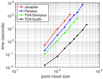
While K[ captures global topological information, there is a major roadblock in using it for data analysis. Figure 1 shows the time to compute PD, the building block of PL and K[ , versus the point cloud size ♣X♣. We compared several popular TDA software: JavaPlex [Tausz et al., 2011], Perseus [Nanda, 2013], the R TDA package [Fasy et al., 2014] with Dionysus [Morozov, 2007] and GUDHI [Maria, 2014] solvers, respectively. The reported time is in seconds on a typical desktop computer for the software to compute 1st persistence diagram. The slopes of these log-log time curves suggest that computation time scales as ♣X♣3 to ♣X♣4 for 1st persistent homology. Objects with more than a few hundred points are computationally prohibitive.
A naive solution to the scalability issue is to sample b points from X to form a sparser point cloud b(X), as suggested in [Chazal et al., 2015b; Chazal et al., 2015a]. Repeating the process s times, we obtain point clouds b1(X) ▷ ▷ ▷ bs(X). A bootstrapping PL function can then be computed as ¯λsb = 1s Pj λbj(X), where the average applies to each PL level separately.
Unfortunately, this bootstrap procedure introduces a loss of resolution. As an example, consider the two point clouds in Figure 2. At the global level (a) they look the same, but zooming in (b) we notice that the top one is made of numerous small rings while the bottom one is simply an annulus.
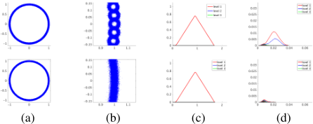
Subsampling globally (c) ignores this difference - justifiably so if one is only concerned with the overall shape of λX, since the finer resolution only contributes minimally to the global PL. Nonetheless, this difference in "topological texture" may be important for classifying or clustering. For better topological data analysis, we need the ability to identify differences in localized topology.
2.2 AMultiresolution Kernel K]
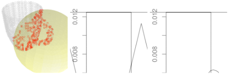
Inspired by multiresolution data analysis, especially the work on local relative homology in [Ahmed et al., 2014], we propose a multiresolution persistent homology description of X to compute localized topology like those in Figure 2(d). To this end consider balls of a particular radius r, which we call the resolution. Let B(c↪ r) = ¶x 2 X : kx - ck r♦ be the set of points in the ball centered at c with radius r. Let λB(c↪r) be the corresponding PL function computed by performing a filtration on B(c↪ r). As an example, Figure 3(left) shows a 3D point cloud of a mug. The ball is shown in yellow, B(c↪ r) shown in red 1 , and λB(c↪r) in Figure 3(mid).
We draw centers c from a probability distribution PC. In this paper, we assume PC is supported on X; that is, each ball must center on one of the data points in X. A simple choice of PC is the uniform distribution over points in X, though a domain expert can design other PC to emphasize certain interesting regions. Our quantity of interest is the expected PL function at resolution r:
1 Actually a subset of B(c↪ r), see section 2.3
When PC is the uniform distribution over X, this quantity is simply ⇡r = 1 ♣X♣ Pc2X λB(c↪r). Let the diameter of X be diam(X) = maxi↪j2X ki - jk. Noting that if r ≥ diam(X), B(c↪ r) = X for all c 2 X, we can establish that 8r ≥ diam(X), ⇡r = λX. Thus r ≥ diam(X) recovers the global PL function. To obtain topological information of X at finer resolutions, we consider L decreasing radii r1 > ▷ ▷ ▷ > rL and compute the corresponding expected PL functions ⇡r1 ↪ ▷ ▷ ▷ ↪ ⇡rL .
Definition 1 The multiresolution persistent homology representation of X at radii r1 ▷ ▷ ▷ rL is (⇡r1 ↪ ▷ ▷ ▷ ↪ ⇡rL ).
We now have all the ingredients to define a multiresolution persistent homology kernel K] . Specifically, we define homology kernel K] between two point cloud objects X and X0 as
where w1↪ ▷ ▷ ▷ ↪wL are nonnegative weights to combine different resolutions. A particularly useful weighting scheme is to set
To understand this scheme, imagine two holes both born at b = 0 and die at d = r1. The inner product (1) between their PLs is r3 1 ◁12. Now imagine two other holes both with b = 0↪ d = ri. Their inner product is r3 i ◁12. The weighting scheme thus scales up the finer resolution so that all resolutions contribute equally to the kernel.
However, the kernel K] (4) is defined without regard to computation. In fact K] is more costly to compute than K[ due to two issues: 1. The expectation inside ⇡ requires enumerating all possible centers c 2 X; 2. B(c↪ r) may still contain many points, making persistent homology software slow (recall Figure 1). We address both issues with sampling next.
2.3 The SMURPHKernel K
The procedure below is carried out independently at each resolution r. We sample m centers c1 ▷ ▷ ▷ cm ⇠ PC. For each center c, we generate j = 1 ▷ ▷ ▷ s bootstrap samples within the ball B(c↪ r). Each bootstrap sample bj(c↪ r) consists of b points sampled with replacement from B(c↪ r). Instead of computing λB(c↪r), we compute λbj(c↪r). The value of b is chosen with computation speed in mind, so that state-of-theart persistent homology software can finish in a reasonable amount of time. We define average persistence landscape (APL), an estimator of ⇡r, as follows:
The superscripts msb remind the reader that ¯λmsb r is subject to three kinds of randomness: m balls, s bootstraps per ball, b points per bootstrap.
To illustrate, we go back to Figure 2. Both the ring-ofrings point cloud and the annulus point cloud in (a) contain one million points. This poses no computational difficulty for ¯λmsb r in (c) and (d) if we choose e.g. b = 300, which is easily handled by state of the art TDA software, and m = 20↪ s = 1.
As another example, Figure 3(right) shows the average persistence landscape on the mug. The most significant persistent homology class (due to the handle) survives the averaging, even though we do not expect every random ball to contain the handle.
Definition 2 The stochastic multiresolution persistent homology representation of X at radii r1 ▷ ▷ ▷ rL is (¯λmsb r1 ↪ ▷ ▷ ▷ ↪ ¯λmsb rL ).
Finally, we define the Stochastic Multi-Resolution Persistent Homology (SMURPH) kernel as:
Note that K is stochastic due to sampling but given the samples it is a positive semi-definite kernel matrix. During test time when one needs to compute the kernel K(Xi↪X⇤ ) between a training object Xi and a new point cloud object X⇤ , it is important that one uses the same representation (¯λmsb r1 ↪ ▷ ▷ ▷ ↪ ¯λmsb rL ) for Xi during training to ensure that the kernel matrix is well-defined.
Algorithm 1 specifies the computation of SMURPH kernel K. If we take the state-of-the-art persistent homology time complexity to be O(b3 ) as indicated by Figure 1, the complexity of Algorithm 1 is O(nLmsb3 + n2 ). We also note that the inner product (1) can be efficiently computed in closed-form since PL is piecewise linear as a consequence of lmax over tent functions. In practice, computing each object's stochastic multiresolution persistent homology representation (¯λmsb r1 ↪ ▷ ▷ ▷ ↪ ¯λmsb rL ) takes a few seconds for modest b in the hundreds.
Algorithm 1 SMURPH Kernel
Input: n point cloud objects X1↪ ▷ ▷ ▷ Xn Parameters: radius scheme (r1↪ ▷ ▷ ▷ ↪ rL), kernel weight scheme (w1↪ ▷ ▷ ▷ ↪wL), center distribution PC, number of centers m, bootstrap sample size b, number of bootstraps s, filtration F . for object X 2 ¶X1 ▷ ▷ ▷ Xn♦ do for resolution r 2 ¶r1 ▷ ▷ ▷ rL♦ do for center i = 1 ▷ ▷ ▷ m do Sample ci ⇠ PC for bootstrap j = 1 ▷ ▷ ▷ s do Sample b points within B(ci↪ r) to form bj(ci↪ r) Apply filtration F on bj(ci↪ r) to compute PL λbj (ci↪ r) end for end for ¯λmsb r = 1 ms Pmi=1 Psj=1 λbj (ci↪ r) end for Represent object X by (¯λmsb r1 ↪ ▷ ▷ ▷ ↪ ¯λmsb rL ) end for Define the n ⇥ n resolution-r kernel matrix as Kr(Xi↪ Xj ) = h¯λmsb r (Xi)↪ ¯λmsb r (Xj)i Output: SMURPH kernel matrix K = PLi=1 wiKri
For theoretical consideration, define the n ⇥ n SMURPH kernel matrix K = [Kij] where Kij = K(Xi↪Xj) for i↪ j = 1↪ ▷ ▷ ▷ ↪ n. Similarly, we define K] = hK] ij i. Following the technique in [Chazal et al., 2015a; 2013], we can show that K approximates K] : under mild conditions E♣♣⇡r - ¯λmsb r ♣♣1 O ⇣ log b b ⌘1◁β ] for some constant β.
This means that ¯λmsb r is an asymptotically unbiased estimator of ⇡r. Furthermore, we can bound E♣♣K] -K♣♣max where ♣♣▷♣♣max is the max matrix norm. If s↪m are of the order ⇣ b log b ⌘2◁β , then E♣♣K] -K♣♣max O ⇣ log b b ⌘1◁β ].
3 Experiments
We present three applications in clustering and classification to demonstrate the potential of the SMURPH kernel.
3.1 Pots and Pans
We demonstrate SMURPH kernel's ability to embed point cloud objects in a meaningful way based on persistent homology features. The dataset consists of 41 point cloud kitchen utensils (e.g. pans, cups, bottles, knives) [Neumann et al., 2013]. We compute SMURPH kernel matrix using a radius of r = 0▷1, m = 20 centers per point cloud, s = 1 samples per center, and a budget of b = 350 points per sample.
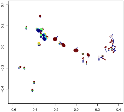
We embed the 41 objects in 2D using kernel PCA on the SMURPH kernel matrix. For better visualization we draw each object centered on its embedding coordinates, see Figure 4. All objects are drawn at the same scale. We identify three salient groups with similar persistent homology in this embedding: (1) mugs with a handle, pots with handles, and long bottles near (-0▷4↪ 0▷2); (2) ladle, knifes, screw drivers near (0▷3↪ 0); (3) small cans near (-0▷4↪-0▷4). We now explain why the grouping is topologically meaningful.
Most objects in the group (1) have handles. We have shown one such mug in Figure 3. Another mug is shown in Figure 5(left). Colors are solely for better visualization. Handles produce large holes in Vietoris-Rips filtration, whose effect is preserved in the average persistence landscape as a tall and long hump. Recall the SMURPH kernel is computed as inner products between these APL functions. The grouping in kPCA embedding space reflects the overall similarity between APL functions. Therefore, objects with handles are grouped close.
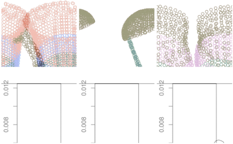
In contrast, objects in group (2), such as the ladle shown in Figure 5(middle), have no intrinsic holes. Their average persistence landscape is almost flat and distinct from group (1). Note their APL is not exactly the zero line - this is an artifact of sampling. To see why, imagine a regular 2D grid of points in a ball B(c↪ r). SMURPH samples b points from the ball. When b is small relative to the number of points in the ball, spurious holes will be created during Vietoris-Rips filtration. In practice, however, this artifact has limited effect and does not prevent kPCA from producing meaningful embedding.
Finally, group (3) reveals an interesting property of SMURPH. First, the three cans are defective and missing the bottom in their point cloud (Figure 5 right), making them similar to the wine glass at (-0▷6↪-0▷2). Second, when SMURPH samples from a ball centered near the bottom, the ball would contain the whole can except the cap. The points in the ball then form a cylinder, which has a large hole. This homology feature will enter APL. In other words, SMURPH reflects both the overall topological structure of the object and that of its parts. We call the latter topological texture. 2 The topological texture of the cans and the wine glass has its own distinct APL signature, and is responsible for group (3).
2 Such topological texture is also responsible for the long bottles, which has no intrinsic 1st order holes, to enter group (1).
3.2 Drusen Detection in Fundus Photography
Drusen are small yellowish hyaline deposits that develop beneath the retinal pigment epithelium. While drusen are natural phenomena that occur with aging, The presence of numerous, larger drusen is predictive of macular degeneration. Some drusen sites form small holes in skeletonized images (Figure 6 right). This suggests SMURPH kernel can help in classifying drusen vs. non-drusen images.
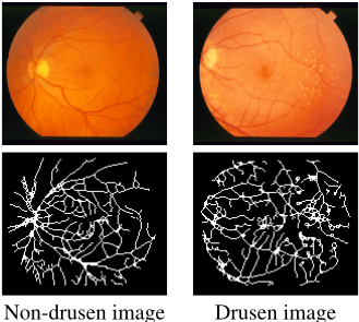
Data. Our sample consists of 67 retinal images, collected as part of the STARE [Hoover and Goldbaum, 2013] project. Of these, 35 have been labeled by experts as images without drusen and 32 as images with drusen. We pre-process the images by first binarizing (setting all non-zero pixel values to 1) and then skeletonizing with MATLAB's bwmorph. Our point cloud is then the coordinates of the nonzero pixels of this skeletonized image. To compute SMURPH kernel, we sample patch centers with a uniform distribution over the point cloud. We choose a resolution level of r = 8 and m = 50, s = 1, b = 300.
Method. We compare SMURPH to two baselines: linear kernel and radial basis function (RBF) kernel. While more sophisticated computer vision processing can undoubtedly enhance the baselines, our goal is to demonstrate the potential of SMURPH without heavy feature engineering. We tune all parameters (regularization C for SVM and bandwidth σ for RBF kernel) using an inner cross validation (CV) inside the outer CV training portion. The tuning grid is C 2 ¶2-7 ↪ 2-6 ↪ ▷ ▷ ▷ ↪ 27 ♦ and σ 2 ¶100 ↪ 101 ↪ ▷ ▷ ▷ ↪ 103 ♦. We feed the kernels to an SVM (kernlab [Karatzoglou et al., 2004]) for classification and report 5-fold CV accuracy.
Results. Table 1 summarizes our results. SMURPH kernel outperforms the linear and RBF kernel baselines, demonstrating that SMURPH captures topological features that help to detect drusen. To assess the significance of our result, we perform a t-test over the accuracy of our classifiers across the CV folds, testing the accuracy of the SMURPH kernel against the RBF kernel and the linear kernel. As reported in Table 1, for either baseline we can reject the null hypothesis that accuracy does not differ at the 0.05 level.
| Kernel | Parameters | Accuracy | p-value |
| SMURPH | C = 32 | 70.2% | - |
|---|---|---|---|
| RBF | C = 2, σ = 10 | 52.2% | 0.040 |
| Linear | C = 2 | 43.3% | 0.007 |
3.3 Human Activity Recognition
We now demonstrate SMURPH kernel's ability to handle point clouds from a state space. In an unsupervised learning setting we show how kernel PCA embeds the n objects; in a supervised learning setting we will use activity as the class label and perform classification.
Data. The "daily and sports activities" data set [Altun et al., 2010] contains sensor data of several everyday activities, among which we choose five representative ones: sitting (A1), walking (A9), running (A12), jumping (A18), and playing basketball (A19). Each activity is performed by 8 people in their own style for five minutes. Each person's data is a time series measured at 25 Hz, for a total of 5⇤60⇤25 = 7500 measurements. Each measurement is 45-dimensional: 5 sensor units placed on torso, right arm, left arm, right leg, and left leg; each sensor unit contains x,y,z accelerometers, x,y,z gyroscopes, and x,y,z magnetometers.
We treat each activity-person combination as an object for a total of n = 5 ⇤ 8 = 40 objects. Each object contains 7500 points. Each point has a time stamp and a 45-dimensional measurement. No processing is performed on the measurements.
Filtration with Timeline. Since each object here is a time series, we present a special filtration design which is of independent interest. A similar filtration has been used to model sequences of natural language paragraphs [Zhu, 2013]. Let the point cloud object be X = ¶x = (t↪ z)♦ where t is the time stamp and z is the measurement vector at time t. Our filtration has two unique steps:
- The ball is defined by t, not by z. That is, p is the uniform distribution over time stamps in X. Once we sample a center in time: c ⇠ Pt, we define the ball B(c↪ r) = ¶x = (t↪ z) 2 X : kt - ck r♦, which is in fact a time interval.
(2) We add a "timeline" (a set of edges) before VietorisRips filtration begins. Within B(c↪ r), we randomly sample b points x1 ▷ ▷ ▷ xb. Sort these points by time so that t1 < ▷ ▷ ▷ < tb. We create the timeline by connecting points (xi↪ xi+1) adjacent in time for i = 1 ▷ ▷ ▷ b - 1. The VietorisRips filtration then proceeds as usual but uses the distance metric on z. The final complex is the union of the timeline and the filtration. All in all, the timeline acts as a pre-existing temporal skeleton to help enhance the filtration. We compute a b ⇥ b distance matrix D where Di↪j = kzi - zjk and set Di↪i+1 = 0 for i = 1 ▷ ▷ ▷ b - 1. Even though D no longer satisfies the triangle inequality it can still serve as a filtration function.
Unsupervised kernel PCA Results. We use two resolution levels: r1 = 125 and r2 = 25 which correspond to 10-second and 2-second intervals. We set the parameters m = 10↪ s = 1↪ b = 100. We compute the 40 ⇥ 40
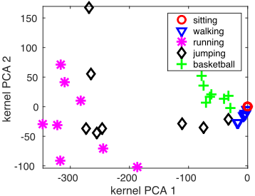
SMURPH kernel matrix with weights w1 = w2 = 1 in (7). We then perform kernel PCA on this kernel matrix to embed the 40 objects in 2D. Figure 7 shows the embedding with annotated activities. Overall the activities form clear clusters. All eight participants' sitting activities are overlapping at the origin. This is expected because each sitting PL is nearly empty. The participants' walking activities are similar and form a tight cluster next to sitting. The cluster of playing basketball is more spread out than walking but tighter than running. We speculate that although basketball is more physical, it also lacks clear periodicity, hence the in-between embedding. Running as a cluster occupies an extreme region in kernel PCA due to both strong activities and clear periodicity. Finally, jumping is the only activity that spread out in the embedding across the eight people. The original data collection in [Altun et al., 2010] instructed people to perform each activity in free style. We suspect that the cluster spread may be attributed to a large variation in how consistently people jumped for five minutes, given that it is a physically demanding activity.
Supervised activity classification. We perform a classification task to predict the five activities. The input is the 40 ⇥ 40 SMURPH kernel matrix. We measure 8-fold CV error, where in each fold we use 7 people (total of 35 activities) as the training data, and leave all 5 activities from one person out as test data. We use SVM light [Joachims, 2008] with our SMURPH kernel. This SVM problem has a single regularization parameter C. We tune C by an inner CV within the first training fold of 7 people. On a parameter grid C 2 ¶10-5 ↪ 10-4 ↪ ▷ ▷ ▷ ↪ 105 ♦, this inner CV selects C = 100. We fix this C for all other outer cross validation folds. The SVM CV accuracy with the SMURPH kernel is 95.0%. In contrast, with a linear kernel the SVM CV accuracy is 62.5%.
4 RelatedWork
This paper is related to but differs from several recent work in topological data analysis:
| multi-resolution | single-resolution | |
|---|---|---|
| kernel | ours | KHNLB15, RHBK15, PHCJS11 |
| non-kernel | AFW14 | Bubenik15, LOC14 |
The closest work AFW14 is the local persistent homology proposed by Ahmed, Fasy, and Wenk [2014]. They computed local relative homology based on PD at various resolutions to compare street maps. SMURPH differs in that we build on PL; we address scalability issue with Monte Carlo; and we construct kernels to enable a much broader range of machine learning applications.
Also closely related are KHNLB15 [Kwitt et al., 2015] and RHBK15 [Reininghaus et al., 2015]'s multi-scale kernel. An important difference is that the "scale" in their multi-scale kernel means different amount of heat diffusion. Therefore, their kernels always describe global topology but with varying amount of smoothing. In contrast SMURPH kernels are defined over varying spatial scales, which allows us to see both global topology and fine-grained "topological texture." In addition our PL-based kernel avoids the need to perform heat diffusion on PDs as they do, and enjoys both conceptual simplicity and computational savings. Both kernels exhibits stability [Bubenik, 2015; Reininghaus et al., 2015] and can be used for machine learning.
Bubenik [2015] pointed out that PL is a Hilbert space. LOC14 [Li et al., 2014] used both PL and PD to measure the global topological distance between point clouds. Their methods did not aim to define kernels, nor did they study multi-resolution. PHCJS11 [Pachauri et al., 2011] proposed a topological kernel for studying Alzheimer's disease. That kernel is based on kernel density estimation within a PD. However, this is a heuristic because a PD is not a 2D Euclidean space. Our paper inherits Chazal et al.'s bootstrap approach and approximates the persistent homology on a full point cloud with that on a random sample [Chazal et al., 2015b; Chazal et al., 2015a]. Their bootstrap approach loses resolution with sampling; our multi-resolution approach ameliorates this issue.
5 Conclusion
We have presented a novel kernel that compares the topology of point cloud objects. Our SMURPH kernel is multiresolutional and can handle large point clouds. It serves as a new bridge between topology and machine learning to encourage further research that can benefit both communities.
There are many ways one can extend SMURPH. The experiments in this paper are only proof-of-concept. One important task is to identify applications where SMURPH, in conjunction with standard kernels, can significantly improve the performance of machine learning applications. Another important task is to go beyond kernel methods and bring the same topological information into probabilistic models.
Acknowledgments The authors thank Fr´ed´eric Chazal and Brittany Fasy for helpful discussions. Support for this research was provided in part by NSF grant IIS 0953219.
@inproceedings{ijcai2016p349,
  title     = {Stochastic Multiresolution Persistent Homology Kernel},
  author    = {Zhu, Xiaojin and Vartanian, Ara and Bansal, Manish and Nguyen, Duy and Brandl, Luke},
  booktitle = {Proceedings of the Twenty-Fifth International Joint Conference on
               Artificial Intelligence, {IJCAI-16}},
  publisher = {AAAI Press / International Joint Conferences on Artificial Intelligence},
  editor    = {Subbarao Kambhampati},
  pages     = {2449--2456},
  year      = {2016},
  month     = {7},
  url       = {https://ijcai.org/proceedings/2016/349},
}
TY - CPAPER TI - Stochastic Multiresolution Persistent Homology Kernel AU - Zhu, Xiaojin AU - Vartanian, Ara AU - Bansal, Manish AU - Nguyen, Duy AU - Brandl, Luke T2 - Proceedings of the Twenty-Fifth International Joint Conference on Artificial Intelligence, IJCAI-16 PB - AAAI Press / International Joint Conferences on Artificial Intelligence PY - 2016 SP - 2449 EP - 2456 UR - https://ijcai.org/proceedings/2016/349 ER -Copied
Machine-readable versions of this paper, for tools and AI agents:





