
Adaptive Variance Reducing for Stochastic Gradient Descent
Proceedings of the Twenty-Fifth International Joint Conference on Artificial Intelligence. Pages 1990-1995.
Abstract
Variance Reducing (VR) stochastic methods are fast-converging alternatives to the classical Stochastic Gradient Descent (SGD) for solving large-scale regularized finite sum problems, especially when a highly accurate solution is required. One critical step in VR is the function sampling. State-of-the-art VR algorithms such as SVRG and SAGA, employ either Uniform Probability (UP) or Importance Probability (IP), which is deficient in reducing the variance and hence leads to suboptimal convergence rate. In this paper, we propose a novel sampling scheme that explicitly computes some Adaptive Probability (AP) at each iteration. Analysis shows that, equipped with AP, both SVRG and SAGA yield provably better convergence rate than the ones with UP or IP, which is confirmed in experiments. Additionally, to cut down the per iteration computation load, an efficient variant is proposed by utilizing AP periodically, whose performance is empirically validated.
- [Beck and Teboulle, 2009] Amir Beck and Marc Teboulle. A fast iterative shrinkage-thresholding algorithm for lin- ear inverse problems. SIAM journal on imaging sciences, 2(1):183-202, 2009.
- [Bottou, 2010] Léon Bottou. Large-scale machine learn- ing with stochastic gradient descent. In Proceedings of COMPSTAT'2010, pages 177-186. Springer, 2010.
- [Chang and Lin, 2011] Chih-Chung Chang and Chih-Jen Lin. LIBSVM: A library for support vector machines. ACM Transactions on Intelligent Systems and Technology, 2:27:1-27:27, 2011.
- [Chen and Rockafellar, 1997] George HG Chen and RT Rockafellar. Convergence rates in forward-backward splitting. SIAM Journal on Optimization, 7(2):421-444, 1997.
- [Csiba et al., 2015] Dominik Csiba, Zheng Qu, and Peter Richtárik. Stochastic dual coordinate ascent with adaptive probabilities. arXiv preprint arXiv:1502.08053, 2015.
- [Defazio et al., 2014] Aaron Defazio, Francis Bach, and Si- mon Lacoste-Julien. Saga: A fast incremental gradient method with support for non-strongly convex composite objectives. In Advances in Neural Information Processing Systems, pages 1646-1654, 2014.
- [Duchi et al., 2011] John Duchi, Elad Hazan, and Yoram Singer. Adaptive subgradient methods for online learn- ing and stochastic optimization. The Journal of Machine Learning Research, 12:2121-2159, 2011.
- [Hastie et al., 2005] Trevor Hastie, Robert Tibshirani, Jerome Friedman, and James Franklin. The elements of statistical learning: data mining, inference and prediction. The Mathematical Intelligencer, 27(2):83-85, 2005.
- [Hu et al., 2009] Chonghai Hu, Weike Pan, and James T Kwok. Accelerated gradient methods for stochastic op- timization and online learning. In Advances in Neural In- formation Processing Systems, pages 781-789, 2009.
- [Johnson and Zhang, 2013] Rie Johnson and Tong Zhang. Accelerating stochastic gradient descent using predictive variance reduction. In Advances in Neural Information Processing Systems, pages 315-323, 2013.
- [Konečnỳ and Richtárik, 2013] Jakub Konečnỳ and Peter Richtárik. Semi-stochastic gradient descent methods. arXiv preprint arXiv:1312.1666, 2013.
- [Konecny et al., 2015] Jakub Konecny, Jie Liu, Peter Richtárik, and Martin Takác. Mini-batch semi-stochastic gradient descent in the proximal setting. 2015.
- [Lewis et al., 2004] David D Lewis, Yiming Yang, Tony G Rose, and Fan Li. Rcv1: A new benchmark collection for text categorization research. The Journal of Machine Learning Research, 5:361-397, 2004.
- [Mahdavi et al., 2013] Mehrdad Mahdavi, Lijun Zhang, and Rong Jin. Mixed optimization for smooth functions. In Ad- vances in Neural Information Processing Systems, pages 674-682, 2013.
- [Nesterov, 1998] Yu Nesterov. Introductory lectures on con- vex programming volume i: Basic course. 1998.
- [Nesterov, 2012] Yu Nesterov. Efficiency of coordinate de- scent methods on huge-scale optimization problems. SIAM Journal on Optimization, 22(2):341-362, 2012.
- [Nesterov, 2013] Yu Nesterov. Gradient methods for mini- mizing composite functions. Mathematical Programming, 140(1):125-161, 2013.
- [Schmidt et al., 2013] Mark Schmidt, Nicolas Le Roux, and Francis Bach. Minimizing finite sums with the stochastic average gradient. arXiv preprint arXiv:1309.2388, 2013.
- [Schmidt et al., 2015] Mark Schmidt, Reza Babanezhad, Mohamed Osama Ahmed, Aaron Defazio, Ann Clifton, and Anoop Sarkar. Non-uniform stochastic average gra- dient method for training conditional random fields. arXiv preprint arXiv:1504.04406, 2015.
- [Shalev-Shwartz and Zhang, 2013a] Shai Shalev-Shwartz and Tong Zhang. Accelerated mini-batch stochastic dual coordinate ascent. In Advances in Neural Information Processing Systems, pages 378-385, 2013.
- [Shalev-Shwartz and Zhang, 2013b] Shai Shalev-Shwartz and Tong Zhang. Stochastic dual coordinate ascent methods for regularized loss. The Journal of Machine Learning Research, 14(1):567-599, 2013.
- [Shalev-Shwartz and Zhang, 2016] Shai Shalev-Shwartz and Tong Zhang. Accelerated proximal stochastic dual coordi- nate ascent for regularized loss minimization. Mathemati- cal Programming, 155(1-2):105-145, 2016.
- [Vitter, 1987] Jeffrey Scott Vitter. Design and analysis of dynamic huffman codes. Journal of the ACM (JACM), 34(4):825-845, 1987.
- [Xiao and Zhang, 2014] Lin Xiao and Tong Zhang. A prox- imal stochastic gradient method with progressive variance reduction. SIAM Journal on Optimization, 24(4):2057- 2075, 2014.
- [Zhao and Zhang, 2014] Peilin Zhao and Tong Zhang. Stochastic optimization with importance sampling. arXiv preprint arXiv:1401.2753, 2014.
References were extracted automatically from the PDF and may contain errors.
Full text extracted automatically from the PDF; figures, tables and equations may differ. The PDF is the version of record.
1 Introduction
Minimization of the Regularized Finite Sum (MRFS) is a class of problems often encountered in Artificial Intelligence and Machine Learning applications. Generally, MRFS has the following form:
where F(w) is the average of finite smooth convex component functions fi(w)↪ i = 1↪ ▷ ▷ ▷ ↪ n, and G(w) is a regularization function, which is convex but may not be smooth. In practice, many Empirical Risk Minimization (ERM) problems [Hastie et al., 2005], such as ridged regression, regularized logistic regression, SVM with smooth loss, and Lasso, can be formulated as (1).
The standard Gradient Decent (GD) method [Chen and Rockafellar, 1997; Nesterov, 1998; Beck and Teboulle, 2009; Nesterov, 2013] for MRFS evaluates the gradients of all n component functions at each iteration, which is computationally prohibitive for large datasets. An alternative strategy is to estimate the full gradient using a solo rfjk in the kth iteration, with fjk drawn from some distribution. This is called Stochastic Gradient Descent (SGD). On the bright side, since no full gradient computation is involved, SGD has low per iteration cost. However, the variance introduced by the stochastic gradient precludes the using of large step-size and leads to a sublinear convergence rate [Hu et al., 2009; Bottou, 2010; Duchi et al., 2011].
⇤Corresponding author
In the past few years, much of the development for stochastic techniques has been driven by the variance reducing (VR) stochastic methods, such as SVRG [Johnson and Zhang, 2013], Mixed Optimization [Mahdavi et al., 2013], S2GD [Koneˇcn`y and Richt´arik, 2013; Konecny et al., 2015], SDCA [Shalev-Shwartz and Zhang, 2013b; 2016; 2013a], SAGA [Defazio et al., 2014], SAG [Schmidt et al., 2013], IProx-SVRG [Xiao and Zhang, 2014], and IProxSDCA [Zhao and Zhang, 2014]. The difference between VR stochastic methods and the vanilla SGD is that the former ensures the expected distance between some modified stochastic gradient and the full gradient diminishes to zero, while the latter will not significantly decrease the variance of the estimation as the algorithm converges. It has been proved that such diminishing variance enables the constant step size as in GD, and guarantees linear convergence in the strongly convex case, e.g. [Xiao and Zhang, 2014]. Thus VR stochastic methods are more efficient than the slow-converging SGD when a highly accurate solution is required.
Generally, VR stochastic methods include two major components: the strategy to adjust the stochastic gradient at each iteration, and the scheme to sample functions or coordinates. For the sampling scheme, Uniform probability (UP) has been widely used in the literature [Johnson and Zhang, 2013; Defazio et al., 2014]. While UP can be implemented efficiently, it is observed that, for many VR algorithms, uniform sampling may result in a suboptimal convergence rate. Several VR methods, e.g. IProx-SVRG [Xiao and Zhang, 2014] and SAGA-NUS [Schmidt et al., 2015], use a non-uniform probability, titled Importance Probability (IP), as remedy. Specifically, the probability that fi is sampled will be proportional to its smoothness parameter.
Recently, Csiba et al. (2015) proposed a variant of SDCA named AdaSDCA and its heuristic version AdaSDCA+. The authors prove that AdaSDCA would converge faster than IProx-SDCA, if the sampling probability takes the solution of another (maybe non-convex) optimization problem at each iteration. However, such solution is in closed form only when all f 0 i s↪ i = 1↪ ▷ ▷ ▷ ↪ n are quadratic, and is numerically difficult to approximate otherwise.
By analyzing the variance of the modified stochastic gradient used in SVRG and SAGA, we propose adaptive sampling schemes for these two methods. Our contributions are listed as follows.
- Our schemes compute the sampling probability in closed form, and can handle any smooth convex loss function, e.g. Logistic Regression, instead of being restricted to quadratic ones.
- By utilizing our adaptive sampling schemes, two VR methods, namely AdaSVRG and AdaSAGA, are proposed as alternatives to SVRG and SAGA respectively. We prove that they have better convergence rate than the originals and confirm our analysis with experiments.
- Moreover, we devise a hybrid method, named HVRG, with low amortized computational cost per iteration. Our experiments show that HVRG enjoys fast convergence as AdaSVRG and AdaSAGA.
2 Preliminaries
2.1 Notations and Assumptions
For x 2 Rd , we use kxk to denote the Euclidean norm and rF(x) to denote the gradient of a function F(·) at x. The proximal operator prox⌘↪G(·) : Rd ! Rd is defined as
We use w⇤ = argminw2Rd P(w) to denote the minimizer of the whole problem. A function f(·) : Rd ! R is said to be L-smooth if for any w1↪ w2 2 Rd
In this paper, the expectations are taken with respect to the random variable jk, which indicates the function fjk is selected in the kth iteration, and are conditioned on all previous iterations, for example
where ¶pi♦ni=1 denotes the distribution of jk, i.e. Pr¶jk = i♦ = pi. For a random vector g, we define V[g] := Ekg - E[g]k2 = E[kgk2 ] - [E[kgk]]2 , which will be critical in our analysis.
2.2 Variance Reducing
Recall that in the kth iteration of SGD, some function fjk is sampled according to ¶pi♦ni=1 , and the variable is updated as
where ⌘k is the step size and g(k) = rfjk (w(k-1) )◁npjk is the stochastic gradient.
For ease of discussion, we assume in this paragraph that G(w) ⌘ 0. Since E[g(k) ] = F(w(k-1) ), we have V[g(k) ] = Ekg(k) k2 - krF(w(k-1) )k2 . However, such term may not converge to zero when w(k-1) ! w⇤ , because while we always have rF(w(k-1) ) ! 0, Ekg(k) k2 does not converge to 0 since rfi(w(k-1) ) 9 0 in general. To counteract the influence of variance, SGD adopts a diminishing step size scheme (usually O( 1k ) or O( 1 pk )) and yields sublinear convergence.
The key to accelerate the convergence is to reduce V[g(k) ] as much as possible, since it obstructs the utilization of large step size. We describe two important techniques designed towards this goal, namely gradient adjustment and non-uniform sampling. Note that they are complementary to each other and should be used jointly.
Gradient Adjustment
Gradient adjustment is a technique that modifies the stochastic gradient to ensure V[g(k) ] ! 0 when w(k-1) ! w⇤ . For example, SVRG maintains a periodically updated variable ˜w and modifies g(k) as
Clearly, g(k) is an unbiased estimation of rF(w(k-1) ), and it is proved that V[g(k) ] ! 0 when w(k-1) ! w⇤ [Johnson and Zhang, 2013]. Another example is SAGA which memorizes the latest computed gradient of each function fi in ↵(k-1) i and uses their average ¯↵(k-1) as a surrogate of rF( ˜w) in SVRG. Thus the updating rule can be written as
Defazio et al. (2014) proves that SAGA ensures V[g(k) ] ! 0 when w(k-1) ! w⇤ . By substituting the modified stochastic gradient (3) and (4) with g(k) in SGD, SVRG and SAGA perform the update (2) to finish the iteration.
Non-Uniform Sampling
While the asymptotic property of V[g(k) ] is improved by gradient adjustment, its value also depends on the sampling probability, see (8). To improve upon UP, Zhao and Zhang (2014) propose to use the Importance Probability (IP) for sampling in SGD and SDCA, which is defined as
where Li is the smoothness parameter of each function fi. Such probability can be used in SVRG and SAGA to improve their bounds on V[g(k) ] [Xiao and Zhang, 2014; Defazio et al., 2014]. Note that IP is left unchanged throughout the iterations and only minimizes some loose upper bound on V[g(k) ]. In the next section, we present an adaptive sampling scheme that directly minimizes V[g(k) ] to reduce the variance to a larger extent.
Algorithm 1 AdaSVRG
Input: w(0) ↪ ⌘↪m↪K Output: w(K) 1: Initialize ˜w =w(0) ↪ ↵(0) i :=rfi(w(0) )↪ i = 1↪ ▷ ▷ ▷ ↪ n 2: ¯↵(0) :=rF( ˜w) 3: for k := 1 to K do 4: Compute the probability ¶p(k) i ♦ni=1 according to (7) 5: Sampling index jk according to ¶p(k) i ♦ni=1 6: g(k) := (rfjk (w(k-1) ) -rfjk ( ˜w))◁np(k) jk + ¯↵(k-1) 7: v(k) :=w(k-1) -⌘g(k) 8: w(k) := Prox⌘↪G(v(k) ) 9: if k mod m = 0 then 10: ˜w := 1m Pm-1 i=0 w(k-i) 11: w(k) := ˜w 12: ¯↵(k) :=rF( ˜w) 13: else 14: ¯↵(k) := ¯↵(k-1) 15: end if 16: end forAlgorithm 2 AdaSAGA
Input: w(0) ↪ ⌘↪K
Output: w(K)
1: Initialize ↵(0)
i :=rfi(w(0) )↪ i = 1↪ ▷ ▷ ▷ ↪ n
- 4: Compute the probability ¶p(k) i ♦ni=1 according to (7)
jk )◁np(k)
- 2: ¯↵(0) := 1n Pni=1 ↵(0) i 3: for k := 1 to K do
- 5: Sampling index jk according to ¶p(k) i ♦ni=1
7: v(k) :=w(k-1) -⌘g(k)
6: g(k) := (rfjk (w(k-1) ) -↵(k-1)
8: w(k) := Prox⌘↪G(v(k) )
i
10: ¯↵(k) := 1n Pni=1 ↵(k) 11: end for
3 Methodology
In the kth iteration, denoting rfjk ( ˜w) with ↵(k-1) jk and rF( ˜w) with ¯↵(k-1) , we can write the stochastic gradient g(k) of SVRG and SAGA in a uniform way:
where β(k) jk :=rfjk (w(k-1) )-↵(k-1) jk and β(k) jk ◁npjk can be regarded as a calibration to ¯↵(k-1) to produce an up-to-date stochastic gradient. We define the Adaptive Probability (AP) as
i.e. fi is sampled with probability proportional to kβ(k) i k. The next lemma shows that AP is the minimizer of V[g(k) ]. Lemma 1. Using the notation in (6), we have that
jk + ¯↵(k-1)
is minimized by taking pi = p(k) i , which is defined in (7).
3.1 Algorithms
Two new algorithms, AdaSVRG and AdaSAGA, are devised by employing AP in SVRG and SAGA respectively. We summarize them in Algorithm 1 and Algorithm 2. Note that when mod(k↪ n) = 1 in AdaSVRG or k = 1 in AdaSAGA, (7) is not well defined since both the numerator and the denominator are zero. However, in such situation, we will have g(k) = ¯↵(k-1) for any jk, and thus we directly set g(k) = ¯↵(k-1) .
The following two lemmas bound V[g(k) ] in AdaSVRG and AdaSAGA respectively. They will be used in the convergence analyses of our algorithms in Section 4.
Lemma 2. Assume that each function fi is Li-smooth and define ¯L := 1n Pni=1 Li. In AdaSVRG, we have
where L(k) A ¯L for each k 2 ¶1 ▷ ▷ ▷m♦.
Remark 1. When UP or IP is used for sampling, similar bound can be obtained, but with L(k) A replaced with maxi Li and ¯L respectively. Since we have L(k) A ¯L maxi Li, our bound is tighter and will lead to faster convergence. Note that L(k) A , ¯L, and maxi Li will appear in the convergence results when the corresponding distribution is used for sampling.
Remark 2. L(k) A is potentially equal to ¯L as AP could be identical to IP, e.g. all fi's are identical. However, we find L(k) A much smaller than ¯L in experiments.
Lemma 3. Assume each function fi is Li-smooth and define ¯L := 1n Pni=1 Li. In AdaSAGA, we have that, in the kth iteration,
for some constant L(k) A , where L(k) A ¯L.
Remark 3. We use this lemma to bound the Lyapunov function (11) when proving the convergence of SAGA. Similar to the previous lemma, when IP or UP is used for sampling, L(k) A degenerates to ¯L and maxi Li respectively, with L(k) A ¯L maxi Li.
3.2 AP vs. IP in SVRG
In this section, we discuss the relation between AP and IP in SVRG and present a concrete example to demonstrate their disparity. As for SAGA, the discussion is similar. Here we assume that every fi is of the form fi(w) := φi(X>i w), where Xi is the non-zero feature vector of the ith sample. We have rfi(w) = φ0i (X>i w)Xi and r2 fi(w) = φ00 i (X>i w)XiX>i .
If we assume each φi(·) to be ↵-smooth, we can compute the smoothness parameter Li of fi
and hence IP:
Now we compute AP
Note that AP degenerates to IP when we substitute each ♣φ0i (X>i w(k) ) -φ0i (X>i ˜w)♣ with its upper bound
However, such upper bound can be rather loose, and AP therefore can be quite different from IP. Consider the case where Xi1 = w⇤ , kXi1 k = kXi2 k, but Xi2 ? w⇤ , and φi2 = φi1 . Additionally, assume that both w(k) and ˜w are close to w⇤ , which happens as the algorithm converges. In such case, both X>i1 w(k) and X>i1 ˜w are close to kw⇤ k2 , but X>i2 w(k) and X>i2 ˜w are close to 0. According to (9) and (10), the sampling probabilities of fi1 and fi2 are equal in IP, but can be far from each other in AP.
4 Analysis
In this section, we show that both AdaSVRG and AdaSAGA converge faster than the originals with IP. The proof utilizes the tightened variance bound we derived in the previous section and is left to the long version of this paper due to limitation of space.
4.1 Convergence Analysis of AdaSVRG
To present the convergence result, let us first define
where θ is some fixed constant. A useful fact about ⇢θ is that, ⇢θ(⌘↪ L1↪m) ⇢θ(⌘↪ L2↪m) for any 0 < ⌘ < 1 4L2 and positive m, if L1 L2. This can be easily checked by computing the derivative of ⇢θ with respect to L. Additionally, auxiliary variables ¶˜w(t) ♦Tt=0 are defined as: ˜w(0) := w(0) , and ˜w(t) := ˜wwhen ˜w is updated for the tth time.
Theorem 1. Assume that F(w) is θ-strongly convex and each fi is Li-smooth. Define ˜L(t) A :=maxi2¶1↪▷▷▷↪m♦ L(tm-i) A , where L(k) A is defined in Lemma 2. Taking m and ⌘t 2 (0↪ 1 4 ˜L(t) A ) such that ⇢θ(⌘t↪ ˜L(t) A ↪m) < 1, we have
Remark 4. Xiao and Zhang (2014) have shown that IProxSVRG has the following convergence result
where ¯ ⌘ 2 (0↪ 1 4¯L ) is some fixed step-size. If we use the same fixed step-size in AdaSVRG, i.e. ⌘t = ¯ ⌘ for each t 2 ¶1 ▷ ▷ ▷ T♦, then we have ⇢θ(¯ ⌘↪ ˜L(t) A ↪m) ⇢θ(¯ ⌘↪ ¯L↪m) and thus Theorem 1 entails that AdaSVRG enjoys a faster convergence. Additionally, it indicates that we can choose a larger step-size in AdaSVRG, e.g. ⌘t = LI ˜L(t) A ¯ ⌘ ≥ ¯ ⌘, which leads to faster convergence in practice. Note that in such case, ⇢θ(⌘t↪ ˜L(t) A ↪m) is still smaller than ⇢θ(¯ ⌘↪ ˜LI ↪m).
4.2 Convergence Analysis of AdaSAGA
Before diving into the convergence theorem of AdaSAGA, we first define φ(k) i := w(k0i-1) for i = 1↪ ▷ ▷ ▷ ↪ n, where k0i k is the last iteration when fi is sampled. We define φ(0) i = w(0) . Following this definition, we have ↵(k-1) i = f 0 i (φ(k-1) i ) for all i = 1↪ ▷ ▷ ▷ ↪ n. Note that φ(k) i is only used for analysis and it is not memorized over iterations. We then define the Lyapunov function T , which is an upper bound of 1 2n⌘ kw-w⇤ k2 due to the convexity of fi:
where ⌘ is some positive constant.
Theorem 2. Assume that F(w) is θ-strongly convex and each fi is Li-smooth, and define ¯L = 1n Pni=1 Li. For AdaSAGA 1 , let T (k) be:
with ⌘ = 1 4¯L being the step size. We have
where k = min¶ 1 2n ↪ θ 8L(k) A ♦ and L(k) A is defined in Lemma 3.
Remark 5. If there is no regularization, i.e. G(w) ⌘ 0, and IP is used for sampling, Schmidt et al. (2015) prove that
where = min¶ 1 3n ↪ θ 8¯L ♦ < 1. Our result is better since (1 - k) (1 - ) for all k = 1↪ ▷ ▷ ▷ ↪m. Besides, it is valid even if G(w) 6= 0. From this theorem, it is clear that w(k) converges to the optimal w⇤ linearly:
5 Efficient Variant
Theorem 1 and 2 suggest that AdaSVRG and AdaSAGA converge faster than SVRG and SAGA respectively. However, exactly computing (7) takes O(nd) operations, which
1 Though unnecessary in practice, some additional uniform samples are needed in our analysis, similar to [Schmidt et al., 2015]
Algorithm 3 HVRG
Input: w0↪ ⌘↪K↪ c↪ ⇢ Output: wK 1: for k := 1 to K do 2: if k mod cn = 1 then 3: Synchronous Update of ↵i's: 4: ↵(k-1) i := rfi(w(k-1) )↪ i = 1↪ ▷ ▷ ▷ ↪ n 5: ¯↵(k-1) := 1n Pni=1 ↵(k-1) i 6: end if 7: if k mod cn = 2 then 8: Compute ¶pi♦ni=1 according to (7) 9: end if 10: Sampling index jk according to ¶pi♦ni=1 11: g(k) := (rfjk (w(k-1) ) -↵(k-1) jk )◁npjk + ¯↵(k-1) 12: v(k) :=w(k-1) - ⌘g(k) 13: w(k) := Prox⌘↪G(v(k) ) 14: ↵(k) i := (rfjk (w(k) ) if i = jk ↵(k-1) i otherwise 15: ¯↵(k) := 1n Pni=1 ↵(k) i 16: Probability Shrinkage: 17: pjk := pjk ◁⇢; for i 6= jk, pi are left unchanged. 18: pj := pj◁ Pni=1 pi↪ j = 1↪ ▷ ▷ ▷ ↪ n 19: end formakes our algorithms less practical when handling large scale problems. To ameliorate this shortcoming, we present a variant called Hybrid Variance Reducing Gradient descent method (HVRG), which computes AP exactly every c epochs (cn iterations). For ease of notation, we suppress the superscripts of ↵i's in this section .
Like AdaSAGA, HVRG keeps auxiliary variables ↵i↪ i = 1↪ ▷ ▷ ▷ ↪ n to store the latest computed gradient for every fi. And like AdaSVRG, it updates all ↵i to rfi(w(k) ) synchronously every c epochs. However, unlike both methods, HVRG exactly computes AP only after updating all ↵i's synchronously, and shrink pjk for the sampled index jk in the kth iteration. We summarize HVRG in Algorithm 3 and discuss the details as follows.
Synchronous Update of ↵i's: When uniform probability is used for sampling, we know from the coupon collector's problem that it takes ⇥(n logn) iterations in expectation for every function fi to be sampled at least once. This means that some function fj will not be visited in ⇥(log n) epochs, nor will the corresponding ↵j be updated. As ¯↵ is kept as the average of all ↵j's, leaving some ↵j out of date potentially undermines the convergence of algorithm. Such situation will get even more severe when non-uniform probability is employed, because the minimum time at which every function is sampled will be further postponed in expectation. To circumvent this pitfall, a periodically full update of all ↵j's is needed.
Shrinkage of pjk : After kth iteration, ↵jk is updated, and the information of rfjk has been incorporated into ¯↵ for estimating of the full gradient in the future iterations. Therefore, the randomness related to fjk is reduced. So we shrink its sampling probability pjk by ⇢, in order to allow other unexplored components to be sampled with higher probability. Csiba et al. (2015) also use similar adaptive sampling method for AdaSDCA+ in dual space.
| Dataset | n | p | λ2 |
|---|---|---|---|
| w7a | 24↪ 692 | 300 | 1◁n |
| ijcnn1 | 49↪ 990 | 22 | 1◁n |
| a9a | 32↪ 561 | 123 | 1◁n |
| covtype | 581↪ 012 | 54 | 1 |
| rcv1 | 20↪ 242 | 47↪ 236 | 10-4 |
| YearPredictionMSD | 463↪ 715 | 90 | 105 ◁n |
Maintenance of Cumulative Distribution Function: In the last line of Algorithm 3, we normalize ¶pi♦ni=1 to make it a distribution. However, such operation takes O(n) operations, which is quite expensive. To alleviate such high cost, we use the Vitter algorithm [Vitter, 1987] to maintain the Cumulative Distribution Function (CDF) of the sampling probability ¶pi♦ni=1 to avoid such normalization procedure. Since we update only one probability per iteration, the maintain operation can be done in O(logn) by this algorithm. Additionally, the sampling operation can be done with the same complexity. An alternative strategy is [Nesterov, 2012] .
Amortized Per Iteration Complexity Updating all ↵i's, exactly computing AP, and constructing the Hoffman tree for CDF take O(nd+n log n) operations, which add O(d+log n) operation to per iteration of HVRG in average, since they are performed only every cn iterations. Addtionally, it takes O(log n) operations to maintain and sample from the CDF as we discussed above. Thus the amortized per iteration complexity is O(d + log n).
6 Experiment
In this section, we present results of several numerical experiments to validate our theoretical analyses of AdaSVRG and AdaSAGA and to show the empirical efficiency of HVRG. Experiments on l2-Logistic Regression, l1l2-Logistic Regression, and Ridge Regression are conducted. We use datasets from LIBSVM [Chang and Lin, 2011] and list their statistics in Table 1. The parameters of the l2-regularization are also included in that table. In our experiments, no normalization is performed on the data. We added an additional feature to all samples to represent the bias term, which is a common practice. SVRG, IProx-SVRG, SAGA 2 , and AdaSDCA+ are included in our experiments for comparison. Since AdaSVRG and AdaSAGA have high per iteration computation load, we only test them on small problems (w7a, ijcnn1, and a9a) to validate our theoretical analysis. The parameter m in SVRG, IProx-SVRG, and AdaSVRG is set to 2n uniformly, as suggested in [Xiao and Zhang, 2014]. We tune the step size (typically from 1 4¯L to 1¯L ) for different methods so that they give the best performance. The parameters c and ⇢ in HVRG are fixed to 5 and 1▷5 respectively. As for initialization, w0 is set to zero in all experiments. We define the log-suboptimality at w as log10 P(w)-P(w⇤ ) P(w0)-P(w⇤ ) and the effective pass as the evaluation of n component gradients. These quantities are used to evaluate the performance of algorithms. Due to the randomness of the algorithms, the reported results are the average of 10 independent trials.
2 SAGA-NUS [Schmidt et al., 2015] is omitted for its poor performance in our experiments
6.1 l2-Logistic Regression
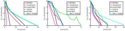
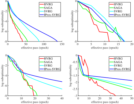
Four datasets are used in l2-Logistic Regression, namely w7a, ijcnn1, a9a, and covtype. We set fi(w) = log(1 + exp(-yiX>i w)) + λ2 2 kwk2 and G(w) = 0, the same as that in [Xiao and Zhang, 2014]. First, we compare the convergence rate of different algorithms in Figure 1. The results show that AdaSAGA and AdaSVRG are the best, conforming to our analysis. We also report the log-suboptimality over the effective pass over the dataset in Figure 2. HVRG either matches or outperforms all the other methods.
6.2 l1l2-Logistic Regression
The rcv1 dataset [Lewis et al., 2004] is used to test the performance of HVRG in l1l2-Logistic Regression, which is a problem with non-zero regularization. We set fi(w) = log(1 + exp(-yiX>i w)) + λ2 2 kwk2 , G(w) = λ1kwk, and λ1 = 10-5 , as suggested in [Xiao and Zhang, 2014]. A critical criterion in such problem is the number of non-zero entries in the variable. We include this quantity in comparison in addition to the log-suboptimality (see Figure 3). HVRG
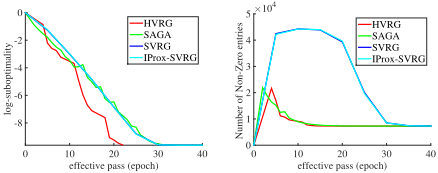
uses the least effective passes to obtain a high accuracy solution and to correctly identify the support of w⇤ .
6.3 Ridge Regression
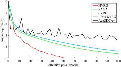
Since AdaSDCA+ can only handle quadratic loss, we include it in comparison by conducting Ridge Regression on the YearPredictionMSD dataset. We set fi(w) = 12 kX>i wyik2 + λ2 2 kwk2 and G(w) = 0. The results are provided in Figure 4. Since the condition number is large in this problem, all algorithms converge slowly. AdaSDCA+ does not seem to converge in primal, although we do find its dual value ascending monotonically. We believe that this has to do with the large condition number. It is clear that HVRG outperforms all the other methods substantially.
7 Conclusion
In this paper, we propose a new adaptive sampling scheme called AP for SVRG and SAGA, and devise two adaptive alternatives, namely AdaSVRG and AdaSAGA, with provably better convergence rate. We validate our analysis with experiments. Additionally, to cut down the per iteration computation load, an efficient variant called HVRG is proposed, whose performance is empirically demonstrated.
Acknowledgment
This work is partially supported by National Natural Science Foundation of China (Grant No: 61472347).
@inproceedings{ijcai2016p284,
  title     = {Adaptive Variance Reducing for Stochastic Gradient Descent},
  author    = {Shen, Zebang and Qian, Hui and Zhou, Tengfei and Mu, Tongzhou},
  booktitle = {Proceedings of the Twenty-Fifth International Joint Conference on
               Artificial Intelligence, {IJCAI-16}},
  publisher = {AAAI Press / International Joint Conferences on Artificial Intelligence},
  editor    = {Subbarao Kambhampati},
  pages     = {1990--1995},
  year      = {2016},
  month     = {7},
  url       = {https://ijcai.org/proceedings/2016/284},
}
TY - CPAPER TI - Adaptive Variance Reducing for Stochastic Gradient Descent AU - Shen, Zebang AU - Qian, Hui AU - Zhou, Tengfei AU - Mu, Tongzhou T2 - Proceedings of the Twenty-Fifth International Joint Conference on Artificial Intelligence, IJCAI-16 PB - AAAI Press / International Joint Conferences on Artificial Intelligence PY - 2016 SP - 1990 EP - 1995 UR - https://ijcai.org/proceedings/2016/284 ER -Copied
Machine-readable versions of this paper, for tools and AI agents:





