
Derivative-Free Optimization of High-Dimensional Non-Convex Functions by Sequential Random Embeddings
Proceedings of the Twenty-Fifth International Joint Conference on Artificial Intelligence. Pages 1946-1951.
© 2016 International Joint Conferences on Artificial Intelligence
Abstract
Derivative-free optimization methods are suitable for sophisticated optimization problems, while are hard to scale to high dimensionality (e.g., larger than 1,000). Previously, the random embedding technique has been shown successful for solving high-dimensional problems with low effective dimensions. However, it is unrealistic to assume a low effective dimension in many applications. This paper turns to study high-dimensional problems with low optimal epsilon-effective dimensions, which allow all dimensions to be effective but many of them only have a small bounded effect. We characterize the properties of random embedding for this kind of problems, and propose the sequential random embeddings (SRE) to reduce the embedding gap while running optimization algorithms in the low-dimensional spaces. We apply SRE to several state-of-the-art derivative-free optimization methods, and conduct experiments on synthetic functions as well as non-convex classification tasks with up to 100,000 variables. Experiment results verify the effectiveness of SRE.
- [Blake et al., 1998] C. L. Blake, E. Keogh, and C. J. Merz. UCI Repository of machine learning databases. [http://www.ics.uci.edu/ ⇠ mlearn/MLRepository.html], 1998. Link
- [Brochu et al., 2010] Eric Brochu, Vlad M. Cora, and Nando de Freitas. A tutorial on bayesian optimization of ex- pensive cost functions, with application to active user modeling and hierarchical reinforcement learning. CoRR, abs/1012.2599, 2010.
- [Bubeck et al., 2009] Sébastien Bubeck, Rémi Munos, and Gilles Stoltz. Pure exploration in multi-armed bandits problems. In Proceedings of the 20th International Con- ference on Algorithmic Learning Theory, pages 23-37, Porto, Portugal, 2009.
- [Bubeck et al., 2011] Sébastien Bubeck, Gilles Stoltz, and Jia Yuan Yu. Lipschitz bandits without the lipschitz con- stant. In Proceedings of the 22nd International Conference on Algorithmic Learning Theory, pages 144-158, Espoo, Finland, 2011.
- [Carpentier and Munos, 2012] Alexandra Carpentier and Rémi Munos. Bandit theory meets compressed sensing for high dimensional stochastic linear bandit. In Proceed- ings of the 15th International Conference on Artificial Intelligence and Statistics, pages 190-198, La Palma, Canary Islands, 2012.
- [Chen et al., 2012] Bo Chen, Rui M. Castro, and Andreas Krause. Joint optimization and variable selection of high-dimensional gaussian processes. In Proceedings of the 29th International Conference on Machine Learning, pages 1423-1430, Edinburgh, Scotland, 2012.
- [Collobert et al., 2006] Ronan Collobert, Fabian Sinz, Jason Weston, and Léon Bottou. Trading convexity for scalabil- ity. In Proceedings of the 23rd International Conference on Machine Learning, pages 201-208, Pittsburgh, Penn- sylvania, 2006.
- [Djolonga et al., 2013] Josip Djolonga, Andreas Krause, and Volkan Cevher. High-dimensional gaussian process ban- dits. In Advances in Neural Information Processing Sys- tems 26, pages 1025-1033, Lake Tahoe, Nevada, 2013.
- [Friesen and Domingos, 2015] Abram L. Friesen and Pe- dro M. Domingos. Recursive decomposition for noncon- vex optimization. In Proceedings of the 24th Interna- tional Joint Conference on Artificial Intelligence, pages 253-259, 2015.
- [Hansen et al., 2003] Nikolaus Hansen, Sibylle D. Müller, and Petros Koumoutsakos. Reducing the time complex- ity of the derandomized evolution strategy with covariance matrix adaptation (CMA-ES). Evolutionary Computation, 11(1):1-18, 2003.
- [Jones et al., 1993] D. R. Jones, C. D. Perttunen, and B. E. Stuckman. Lipschitzian optimization without the lipschitz constant. Journal of Optimization Theory and Applica- tions, 79(1):157-181, 1993.
- [Kandasamy et al., 2015] Kirthevasan Kandasamy, Jeff Schneider, and Barnabás Póczos. High dimensional bayesian optimisation and bandits via additive models. In Proceedings of the 32nd International Conference on Machine Learning, pages 295-304, Lille, France, 2015.
- [Kawaguchi et al., 2015] Kenji Kawaguchi, Leslie Pack Kaelbling, and Tomás Lozano-Pérez. Bayesian optimiza- tion with exponential convergence. In Advances in Neu- ral Information Processing Systems 28, pages 2791-2799, Montreal, Canada, 2015.
- [Munos, 2014] Rémi Munos. From bandits to Monte-Carlo Tree Search: The optimistic principle applied to optimiza- tion and planning. Foundations and Trends in Machine Learning, 7(1):1-130, 2014.
- [Pintér, 1996] János D. Pintér. Global Optimization in Ac- tion, Continuous and Lipschitz Optimization: Algorithms, Implementations and Applications. Nonconvex Optimiza- tion and Its Applications. Kluwer Academic Publishers, Dordrecht, Boston, London, 1996.
- [Qian and Yu, 2016] Hong Qian and Yang Yu. Scaling si- multaneous optimistic optimization for high-dimensional non-convex functions with low effective dimensions. In Proceedings of the 30th AAAI Conference on Artificial In- telligence, Phoenix, AZ, 2016.
- [Snoek et al., 2012] Jasper Snoek, Hugo Larochelle, and Ryan P. Adams. Practical bayesian optimization of ma- chine learning algorithms. In Advances in Neural Infor- mation Processing Systems 25, pages 2960-2968, Lake Tahoe, Nevada, 2012.
- [Vapnik, 2000] Vladimir Vapnik. The Nature of Statistical Learning Theory. Springer Science & Business Media, 2000.
- [Wang et al., 2013] Ziyu Wang, Masrour Zoghi, Frank Hut- ter, David Matheson, and Nando De Freitas. Bayesian op- timization in high dimensions via random embeddings. In Proceedings of the 23rd International Joint Conference on Artificial Intelligence, pages 1778-1784, Beijing, China, 2013. IJCAI
- [Yu et al., 2016] Yang Yu, Hong Qian, and Yi-Qi Hu. Derivative-free optimization via classification. In Proceed- ings of the 30th AAAI Conference on Artificial Intelligence, Phoenix, AZ, 2016.
- [Yuille and Rangarajan, 2001] Alan L. Yuille and Anand Rangarajan. The concave-convex procedure (CCCP). In Advances in Neural Information Processing Systems 14, pages 1033-1040, Vancouver, British Columbia, Canada, 2001.
- [Zhang et al., 2013] Lijun Zhang, Mehrdad Mahdavi, Rong Jin, Tianbao Yang, and Shenghuo Zhu. Recovering the optimal solution by dual random projection. In Proceed- ings of the 26th Conference on Learning Theory, pages 135-157, Princeton, NJ, 2013.
References were extracted automatically from the PDF and may contain errors.
Full text extracted automatically from the PDF; figures, tables and equations may differ. The PDF is the version of record.
1 Introduction
Solving sophisticated optimization problems plays an important role in artificial intelligence. Let f : RD ! R be a function of which we assume that a global minimizer x⇤ always exists. An optimization problem can be formally written as
We assume that the optimization problems discussed in this paper are deterministic, i.e., every call of f(x) returns the same value for the same x.
In this paper, we focus on derivative-free optimization methods, which regard f as a black-box function that can only be evaluated point-wisely, i.e., they perform optimization based on the function values f(x) for the sampled solutions and other information like gradient is not used. Because these methods do not rely on derivatives, they are suitable for optimization problems that are, e.g., with many local optima, non-differentiable, and discontinuous, which are often encountered in a wide range of applications. The performance of a derivative-free optimization algorithm can be evaluated by the simple regret [Bubeck et al., 2009], i.e., given n function evaluations, for minimization,
⇤This research was supported by the NSFC (61375061, 61223003), Foundation for the Author of National Excellent Doctoral Dissertation of China (201451), and 2015 Microsoft Research Asia Collaborative Research Program.
where x(n) 2 RD is the solution with the lowest function value found by the algorithm when the budget of n function evaluations is used up. The simple regret measures the difference between the best function value found by the algorithm and the minimum of f .
Many derivative-free optimization methods have been designed under various principles. They can be roughly categorized into three kinds: model-based methods, deterministic Lipschitz optimization methods and meta-heuristic search. Model-based methods, such as Bayesian optimization methods [Brochu et al., 2010; Snoek et al., 2012; Kawaguchi et al., 2015] and classification-based methods [Yu et al., 2016], learn a model from the solutions and the model is then applied to guide sampling of solutions for the next round. Deterministic Lipschitz optimization methods need Lipschitz continuity assumption on f, such as [Jones et al., 1993; Pint´er, 1996; Bubeck et al., 2011; Munos, 2014]. Meta-heuristic search is designed with inspired heuristics, such as evolutionary strategies [Hansen et al., 2003].
Problem. Almost all derivative-free methods are effective and efficient in low-dimensional problems (usually less than 100 dimensions), but are hard to scale to high dimensionality (say, larger than 1,000 dimensions). This is mainly due to either the low convergence rate in high-dimensional space, thus unbearably many iterations are required; or the per-iteration computational cost is very high in high-dimensional space, thus it is unbearable for finishing a few iterations; or even both of the reasons. The unsatisfactory scalability is one of the main bottlenecks of these methods.
Related Work. Recently, there are some studies focusing on improving the scalability of derivative-free methods. The two major directions are decomposition and embedding.
Decomposition methods extract sub-problems from the original optimization problem, and by solving the subproblems the original problemwill be solved. In [Kandasamy et al., 2015], additive functions were considered, i.e., the function value f(x) is the sum of several sub-functions with smaller dimensions, and there is no variable overlaps between any two sub-functions. In [Kandasamy et al., 2015], via employing a Bayesian optimization method, it was shown that using the additive structure can effectively accelerate the Bayesian optimization method. In [Friesen and Domingos, 2015], a recursive decomposition method was proposed for approximately locally decomposable problems. These methods, however, rely on the (mostly axis-parallel) decomposability, which may restrict their applications.
Embedding methods assume that in the high-dimensional space, only a small subspace effects the function value. Therefore, optimization only in the effective subspace can save a lot of efforts. In [Carpentier and Munos, 2012], compressed sensing was employed to deal with linear bandit problems with low-dimensional effective subspaces. In [Chen et al., 2012], a variable selection method was proposed to identify the effective axis-parallel subspace. In [Djolonga et al., 2013], a low-rank matrix recovery technique was employed to learn the effective subspace. In [Wang et al., 2013; Qian and Yu, 2016], the random embedding based on the random matrix theory was employed to identify the underlying linear effective subspace. However, real-world problems may not have a clear effective subspace, also it is hard to verify the existence of the effective subspace.
Our Contributions. In this paper, we study highdimensional problems with low optimal "-effective dimensions (see Definition 1). In these problems, any (linear transformed) variable is allowed to effect the function value, however, only a small linear subspace has a large impact on the function value, and the orthogonal complement subspace makes only a small bounded effect.
Firstly, we characterize the property of random embedding for this kind of problems. We find that, given optimal "- effective dimension, single random embedding bears 2" embedding gap. Note that this embedding gap cannot be compensated by the optimization algorithm.
We then propose the sequential random embeddings (SRE) to overcome the embedding gap. SRE applies the random embedding several times sequentially, and in each subspace, SRE employs an optimization algorithm to reduce the residue of the previous solution. Therefore, SRE can also be viewed as a combination of decomposition and embedding, as each random embedding defines a sub-problem. We also disclose the condition under which SRE could improve the optimization quality for a large class of problems.
In experiments, we apply SRE to several state-of-the-art derivative-free optimization methods, and conduct experiments on synthetic functions as well as classification tasks using the non-convex Ramp loss. Experiment results show that SRE can significantly improve the performance of the optimization methods in high-dimensional problems. Moreover, comparing with previous related studies where testing functions are mostly up to 1,000 variables, the derivative-free methods with SRE are tested for up to 100,000 variables, in real-world data sets.
The consequent sections respectively introduce the optimal "-effective dimension problems and present the property of random embedding, describe the proposed SRE technique as well as its theoretical property, present the empirical results, and finally conclude the paper.
2 Optimal "-Effective Dimension and Random Embedding
Optimal "-Effective Dimension
Effective dimension defined in [Wang et al., 2013] requires the existence of a non-effective linear subspace, which has exactly zero effect on the function value. It is often unrealistic to make such an assumption. We thus make a relaxation to this assumption as the optimal "-effective dimension in Definition 1.
Note that a function with optimal "-effective dimension can have no low-dimensional effective subspace according to the definition given in [Wang et al., 2013], i.e., no linear subspace that has exactly zero effect on the function value. Instead, it has a linear subspace that makes at most " contribution to the function value. Therefore, this kind of problems may still be efficiently tackled when " is not so large.
DEFINITION 1 (Optimal "-Effective Dimension)
For any " > 0, a function f : RD ! R is said to have an "-effective subspace V", if there exists a linear subspace V" ✓ RD s.t. for all x 2 RD , we have ♣f(x) - f(x")♣ ", where x" 2 V" is the orthogonal projection of x onto V". Let V" denote the collection of all the "-effective subspaces of f, and dim(V) denote the dimension of a linear subspace V. We define the optimal "-effective dimension of f as d" = minV"2V" dim(V").
In the definition above, it should be noted that " and d" are related variables, commonly, a small d" implies a large ", while a small " implies a large d".
Random Embedding
Given the definition of optimal "-effective dimension, Lemma 1 below shows the effect of random embedding for such functions. For simplicity, let N denote the Gaussian distribution with zero mean and σ2 variance.
LEMMA 1
Given a function f : RD ! R with optimal "-effective dimension d", and any random matrix A 2 RD⇥d (d ≥ d") with independent entries sampled from N, then, with probability 1, for any x 2 RD , there exists y 2 Rd s.t. ♣f (x) - f (Ay)♣ 2".
Let Φ 2 RD⇥d" be a matrix whose columns form a standard orthonormal basis for V". For any x" 2 V", there exists c 2 Rd" s.t. x" = Φc. Let us for now assume that
Proof. We borrow the idea of constructing such y as in [Wang et al., 2013]. Since f has the optimal "-effective dimension d", there exists an "-effective subspace V" ✓ RD s.t. dim(V") = d". Besides, any x 2 RD can be decomposed as x = x" + x?" , where x" 2 V", x?" 2 V ? " and V ? " is the orthogonal complement of V". By the definition of "- effective subspace, we have ♣f(x) - f(x")♣ ". Hence, it suffices to show that, for any x" 2 V", there exists y 2 Rd s.t. ♣f(x") - f(Ay)♣ ".
Φ>A has rank d". If rank(Φ>A) = d", there must exist y 2 Rd s.t. (Φ>A)y = c, because rank(Φ>A) = rank([Φ>A↪ c]). The orthonormal projection of Ay onto V" is given by ΦΦ>Ay = Φc = x". Thus, Ay = x"+˜x where ˜x 2 V ? " for x" is the orthonormal projection of Ay onto V". Since Ay 2 RD , by the definition of "-effective subspace, we have ♣f(x") - f(Ay)♣ ", and thus ♣f(x) - f(Ay)♣ 2". Similar to the proof of Theorem 2 in [Wang et al., 2013],
we have that rank(Φ>A) = d" with probability 1. ⌅
Lemma 1 implies that, given a random embedding matrix A 2 RD⇥d , for any minimizer x⇤ 2 RD , there exists ˜ y 2 Rd such that f(A˜ y)-f(x⇤ ) 2". Note that this embedding gap grows twice as fast as ".
Optimization with Random Embedding
Via random embedding, current derivative-free optimization algorithms can be applied to solve high-dimensional optimization problems by running in a low-dimensional solution space. Given a high-dimensional function f and a random matrix A 2 RD⇥d , we construct a new optimization function g(y) = f(Ay), where the solution space for g only has a dimension d. Note that every solution is evaluated by mapping back to the original high-dimensional space.
For functions with a low optimal "-effective dimension, we can bound the gap between the optimal function values of g and f based on Lemma 1, which is stated in Theorem 1. We omit the proof since it can be verified directly.
THEOREM 1
Given a function f : RD ! R with optimal "-effective dimension d", and a random matrix A 2 RD⇥d (d ≥ d") with independent entries sampled fromN, let x⇤ be a global minimizer of f and g(y) = f(Ay) where y 2 Rd , then, with probability 1, we have
We then look into the simple regret of a derivative-free optimization algorithm using a random embedding. The optimization algorithm works in the low-dimensional space, and usually, it can only approximate the optimal solution, thus there is a gap between the found solution ˜ y and the optimal solution in the low-dimensional space infy2Rd g(y). This approximation gap is related to dimension size, function complexity, and optimization budget. We assume that the approximation gap is upper bounded by ✓. Furthermore, as disclosed by Theorem 1, there exists an embedding gap 2", which cannot be compensated by the optimization algorithm. We then have that the simple regret of the algorithm is upper bounded by the approximation gap and the embedding gap,
3 Sequential RandomEmbeddings
From Eq.(1), in order to improve the simple regret, i.e., g( ˜ y) - f(x⇤ ), we need to reduce the approximation gap and the embedding gap. Unfortunately, this two factors are conflicting: In order to reduce the embedding gap, we need to use a large d" to trade for a smaller ", but with a large d", the optimization algorithm needs to deal with more dimensions, which will badly increase the approximation gap.
- Let Si = ¶A(i)y ♣ y 2 Rd ♦ denote the subspace defined by the random matrix, where i = 1↪ ▷ ▷ ▷ ↪m. In spired by [Zhang et al., 2013], we propose the technique of sequentially using multiple random embeddings to reduce the embedding gap while keeping the approximation gap almost unaffected:
- ÷ In the first step, it generates a random matrix A(1) which defines a subspace S1, and applies the chosen optimization algorithm to find a near-optimal solution in the subspace, i.e., ˜ y1 = argminy f(A(1)y). Let ˜x2 = A(1) ˜ y1 be the highdimensional solution.
- ÷ In the second step, it generates another random matrix A(2) which defines a subspace S2, and applies the algorithm to optimize the residue of the current solution ˜x2 in the subspace, i.e., ˜ y2 = argminy f(˜x2 +A(2)y). Then update the current solution ˜x3 = ˜x2 + A(2) ˜ y2.
- ÷ In the following steps, it acts like the second step that performs the optimization to reduce the residue.
By this simple sequence of applying random embeddings, we show that, for a large class of functions with optimal "-effective dimension, an upper bound of the solution gap f(˜xi) - f(x⇤ ) reduces as the step i increases.
Theoretical Property
Let ˜x1 = 0, and k · k represent k · k2 for simplicity. In the step i of the sequential random embeddings, the residue solution to be approximated is x⇤ - ˜xi, let ˆxi be the orthonormal projection of x⇤ - ˜xi onto the subspace Si. Thus, we call kˆxik◁kx⇤ - ˜xik as the embedding ratio which is smaller than 1, and kˆxi -A(i) ˜ yik◁kˆxik as the optimization ratio for this step. We show in Proposition 1 that, when the optimization ratio is less than a fraction of the embedding ratio, the solution is closer to the optimal solution.
PROPOSITION 1
Given f 2 F, and a sequence of random matrices ¶A(i) ♦i ✓ RD⇥d (d ≥ d") each with independent entries sampled from N, for all i = 1↪ ▷ ▷ ▷ ↪m, if
Proof. For any i = 1↪ ▷ ▷ ▷ ↪m, since ˆxi is the orthonormal projection of x⇤ - ˜xi onto Si, we have that
where the last inequality is by kA(i) ˜ yik - kˆxik kˆxi - A(i) ˜ yik.
We then consider a very general class of problems, i.e., functions with local H¨older continuity as in Definition 2.
DEFINITION 2 (Local H¨older Continuity)
Intuitively, Definition 2 means that the rate of increase of f around x⇤ is bounded. Note that a function with local H¨older continuity can have many local optima, or non-differentiable.
For any function with local H¨older continuity, since
Proposition 1 implies that the sequential random embeddings can reduce this upper bound in a mild condition.
Less Greedy
By the method of sequential random embeddings (SRE), each sub-problem in the subspace is solved greedily. However, a perfect solution for one sub-problem may not be good globally, and once an unsatisfied solution is found, it is hard to be corrected by the later solutions because of the greedy process. Therefore, we further introduce a withdraw variable ↵ to the previous solution such that it is possible to eliminate the previous solution if necessary, and the optimization problem in each step becomes
Since derivative-free optimization methods are employed, which make few requirements on the optimization problems, we can simply let the algorithm optimize ↵ together with y.
The full algorithm named SRE is depicted in Algorithm 1. Given a derivative-free optimization algorithm M, in each step of SRE, M optimizes a low-dimensional function gi(y) as defined in line 4, and returns the best solution as well as the withdraw variable found byM (line 5). Finally, the best solution throughout the procedure is returned as the output.
4 Experiments
For the practical issues in experiments, we set the random matrix A 2 RD⇥d with independent entries sampled from N(0↪ 1◁d), and we consider the high-dimensional solution space X = [-u↪ u]D instead of RD and low-dimensional solution space Y = [-l↪ l]d instead of Rd with u↪ l > 0 for simplicity. To implement the derivative-free algorithm in Y, note that there may exist y0 2 Y s.t. Ay0 ◁2 X and thus f cannot be evaluated at point Ay0 . To tackle this problem, we employ Euclidean projection, i.e., Ay0 is projected to X when it is outside X by PX (Ay0 ) = argminx2X kx-Ay0 k2. Let f(PX(Ay0 ))+kPX(Ay0 )-Ay0 k1 be the function value of Algorithm 1 Sequential Random Embeddings (SRE)
Input:
Objective function f;
Derivative-free optimization algorithmM;
Number of function evaluation budget n;
Upper bound of the optimal "-effective dimension d; Number of sequential random embeddings m.
Procedure:
- 1: ˜x1 = 0.
- 2: for i = 1 to mdo
- 3: Sample a randommatrixA(i) 2RD⇥d withAi↪j ⇠N.
- 4: Apply M to optimize the low-dimensional function gi(y) = f(↵˜xi +A(i)y) with nm function evaluations.
- 5: Obtain the solution ˜ yi and ↵i for gi(y) byM.
- 6: ˜xi+1 = ↵i˜xi +A(i) ˜ yi .
- 7: end for
- 8: return argmini=2↪▷▷▷↪m+1 f(˜xi).
Ay0 where Ay0 ◁2 X. Let [x]i denote the i-th coordinate of x. Since X = [-u↪ u]D , the closed form of Euclidean projection is [PX(Ay)]i = -u if [Ay]i < -u; [PX(Ay)]i = [Ay]i if -u [Ay]i u; and [PX (Ay)]i = u otherwise.
We employ three state-of-the-art derivative-free optimization methods: IMGPO [Kawaguchi et al., 2015], which is a combination of Bayesian optimization and optimistic optimization, CMAES [Hansen et al., 2003], which is a representative of evolutionary algorithms, and RACOS [Yu et al., 2016], which is a model-based optimization algorithm proposed recently. All implementations of them are by their authors. We also employ random search as a reference baseline.
When we apply the single random embedding with these optimization algorithms, we denote by the prefix "RE-", and when we apply the SRE, we denote by the prefix "SRE-". Thus we have combinations including RE-IMGPO, RE-CMAES, RE-RACOS, SRE-IMGPO, SRE-CMAES, and SRE-RACOS.
On Synthetic Functions
We first test the algorithms on two synthetic testing functions. Based on the convex Sphere function and the highly nonconvex Ackley function, we construct the high-dimensional Sphere function and Ackley function to meet the optimal "- effective dimension assumption.
The high-dimensional Sphere function is constructed as
where the dimensions except the first 10 ones have limited impact on the function value. The high-dimensional Ackley function is similarly constructed as
Noted that the optimal solutions of these functions are (0▷2↪ ▷ ▷ ▷ ↪ 0▷2), in order to avoid the all-zero optimal solution which is in all the linear subspaces. These functions are minimized within the solution space X = [-1↪ 1]D . We set Y = [-1↪ 1]d ↪ ↵ 2 [-1↪ 1]. Each algorithm is run 30 times independently, and the average performance is reported.
On the number of random embeddings m. We first study the effect of SRE iteration number m, i.e., the number of sequential random embeddings. We choose D = 10000, set the total number of function evaluations n = 10000 and the subspace size d = 10, and choose the number of sequential random embeddings m = ¶1↪ 2↪ 5↪ 8↪ 10↪ 20♦. When m = 1, algorithms with SRE degenerate into algorithms with RE. The achieved objective function values are shown in Figure 1.
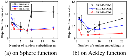
Figure 1 (a) and (b) show that, if the total number of function evaluations is fixed, we should choose a compromised value for m. Because if m is large then the budget for each step of SRE is limited, and if m is small then the steps in SRE is limited, and both of them can lead to unsatisfied optimization performance.
On subspace dimension d. To study how low-dimensional size d affects optimization performance, we only adopt the algorithms with SRE (SRE-IMGPO, SRE-CMAES, SRERACOS). We choose D = 10000, set the total number of function evaluations n = 10000, choose d = ¶1↪ 5↪ 8↪ 10↪ 12↪ 15↪ 20♦, and set the number of sequential random embeddings m = 5. The achieved objective function values are shown in Figure 2.
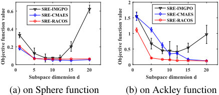
Figure 2 (a) and (b) show that, for algorithms with SRE, in most cases the closer the d to d" the better the optimization performance, indicating that a good estimate of the optimal "-effective dimension is desirable. Besides, we can observe that, even if d < d" = 10 but close to d", the performances of algorithms with SRE are still satisfied.
On scalability. We then study the scalability w.r.t. the solution space dimensions D, we choose D =
¶100↪ 500↪ 1000↪ 5000↪ 10000♦, set the total number of function evaluations n = 10000 for all algorithms, set d = 10 for algorithms with RE and SRE, and set the number of sequential random embeddings m = 5 for algorithms with SRE. The achieved objective function values are shown in Figure 3.
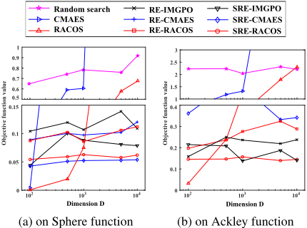
Figure 3 (a) and (b) show that the algorithms with SRE have the lowest growing rate, while the algorithms without RE have the highest growing rate as the dimension increases, indicating that SRE can scale the derivative-free algorithms to high-dimensional problems better than the compared algorithms.
On convergence rate. To study the convergence rate w.r.t. the number of function evaluations, we set D = 10000, and set the total number of function evaluations n = ¶2000↪ 4000↪ 6000↪ 8000↪ 10000♦, set low-dimensional size d = 10 for RE as well as SRE, and set m = 5 for SRE. The achieved objective function values are shown in Figure 4.
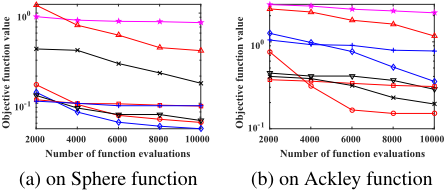
Figure 4 (a) and (b) show that, in most cases, algorithms with SRE reduce the objective function value with the highest rate, while the algorithms without RE reduce the objective function value with the lowest rate, indicating that algorithms with SRE converge faster in general than the others.
On Classification with Ramp Loss
We finally study on a classification task with Ramp loss [Collobert et al., 2006]. The Ramp loss is defined as Rs(z) =
H1(z) - Hs(z) with s < 1, where Hs(z) = max¶0↪ s - z♦ is the Hinge loss with s being the Hinge point. The task is to find a vector w and a scalar b to minimize
f (w↪ b) = 12 kwk22 + C PL`=1 Rs (y`(w>v` + b)), where v` is the training instance and y` 2 ¶-1↪+1♦ is its label. This objective function is similar to that of support vector machines (SVM) [Vapnik, 2000], but the loss function of SVM is the Hinge loss. Due to the convexity of the Hinge loss, the number of support vectors increases linearly with the number of training instances in SVM, which is undesired with respect to scalability. While this problem can be relieved by employing the Ramp loss [Collobert et al., 2006].
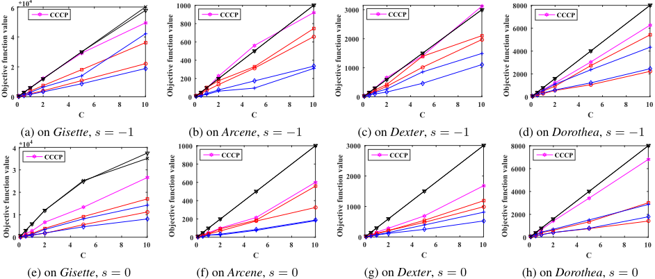
The applied algorithms here are RE-IMGPO, RE-CMAES, RE-RACOS, SRE-IMGPO, SRE-CMAES, SRE-RACOS and the concave-convex procedure (CCCP) [Yuille and Rangarajan, 2001] which is a gradient-based non-convex optimization approach for objective functions that can be decomposed into convex sub-function plus concave sub-function. We employ four binary class UCI datasets [Blake et al., 1998], Gisette, Arcene, Dexter and Dorothea. The feature dimension (D) of which are 5 ⇥ 103 ↪ 104 ↪ 2 ⇥ 104 , and 105 , respectively. Since there are two hyper-parameters in the optimization formulation, i.e., C and s, to study the effectiveness of the compared algorithms under different hyper-parameters, we test s 2 ¶-1↪ 0♦ and C 2 ¶0▷1↪ 0▷5↪ 1↪ 2↪ 5↪ 10♦. We set d = 20, the number of function evaluations n = 3D, and X = [-10↪ 10]D ↪ Y = [-10↪ 10]d ↪ ↵ 2 [-10↪ 10] for all applied algorithms except for CCCP. For CCCP, we set X = [-10↪ 10]D and let CCCP run until it converges. For algorithms with SRE, we set the number of sequential random embeddings m = 5. Each randomized algorithm is repeated 30 times independently. Since we focus on the optimization performance, the achieved objective function values on each dataset are reported in Figure 5.
We should note that, in Figure 5, the lines of RE-IMGPO often overlap with those of SRE-IMPGO, and in sub-figure
(c), the line of CCCP overlaps with SRE-IMPGO. As shown in Figure 5, except in the dataset Arcene, algorithm with SRE has the best performance for any setting of s and C. And in the dataset Arcene, algorithm with RE achieves the best performance. This verifies the effectiveness of SRE and RE, and indicates that SRE is more effective than RE. Comparing CCCP to the derivative-free algorithms with SRE, we can observe that the objective function value of CCCP is approximately as twice as that of the best algorithm with SRE. This implies that algorithms with SRE can be significantly better than CCCP with respect to optimization performance.
5 Conclusion
This paper investigates high-dimensional problems in a more general situation compared with previous works, i.e., all variables can be effective to the function value, while many of them only have a small bounded effect. We define this kind of problems as functions with a low optimal "-effective dimension, and find that, for this kind of problems, single random embedding makes 2" loss that can not be compensated by the following optimization algorithm. Thus, we propose the sequential random embeddings (SRE) that employ the random embedding several times, and the condition under which SRE can reduce the embedding loss strictly in each step of SRE is disclosed. To study the effectiveness of SRE, we apply SRE to several state-of-the-art derivative-free algorithms. Experiment results on optimization testing functions and classification with the non-convex Ramp loss (where the number of variables are up to 100,000) indicate that SRE can scale these derivative-free methods to high-dimensional problems significantly.
@inproceedings{ijcai2016p278,
  title     = {Derivative-Free Optimization of High-Dimensional Non-Convex Functions by Sequential Random Embeddings},
  author    = {Qian, Hong and Hu, Yi-Qi and Yu, Yang},
  booktitle = {Proceedings of the Twenty-Fifth International Joint Conference on
               Artificial Intelligence, {IJCAI-16}},
  publisher = {AAAI Press / International Joint Conferences on Artificial Intelligence},
  editor    = {Subbarao Kambhampati},
  pages     = {1946--1951},
  year      = {2016},
  month     = {7},
  url       = {https://ijcai.org/proceedings/2016/278},
}
TY - CPAPER TI - Derivative-Free Optimization of High-Dimensional Non-Convex Functions by Sequential Random Embeddings AU - Qian, Hong AU - Hu, Yi-Qi AU - Yu, Yang T2 - Proceedings of the Twenty-Fifth International Joint Conference on Artificial Intelligence, IJCAI-16 PB - AAAI Press / International Joint Conferences on Artificial Intelligence PY - 2016 SP - 1946 EP - 1951 UR - https://ijcai.org/proceedings/2016/278 ER -Copied
Machine-readable versions of this paper, for tools and AI agents:





