
Towards Convolutional Neural Networks Compression via Global Error Reconstruction
Proceedings of the Twenty-Fifth International Joint Conference on Artificial Intelligence. Pages 1753-1758.
© 2016 International Joint Conferences on Artificial Intelligence
Abstract
In recent years, convolutional neural networks (CNNs) have achieved remarkable success in various applications such as image classification, object detection, object parsing and face alignment. Such CNN models are extremely powerful to deal with massive amounts of training data by using millions and billions of parameters. However, these models are typically deficient due to the heavy cost in model storage, which prohibits their usage on resource-limited applications like mobile or embedded devices. In this paper, we target at compressing CNN models to an extreme without significantly losing their discriminability. Our main idea is to explicitly model the output reconstruction error between the original and compressed CNNs, which error is minimized to pursuit a satisfactory rate-distortion after compression. In particular, a global error reconstruction method termed GER is presented, which firstly leverages an SVD-based low-rank approximation to coarsely compress the parameters in the fully connected layers in a layer-wise manner. Subsequently, such layer-wise initial compressions are jointly optimized in a global perspective via back-propagation. The proposed GER method is evaluated on the ILSVRC2012 image classification benchmark, with implementations on two widely-adopted convolutional neural networks, i.e. the AlexNet and VGGNet-19. Comparing to several state-of-the-art and alternative methods of CNN compression, the proposed scheme has demonstrated the best rate-distortion performance on both networks.
- [A. Krizhevsky and Hinton, 2012] I.
- Sutskever A. Krizhevsky and G. Hinton. Imagenet classifica- tion with deep convolutional neural networks. In NIPS, pages 1097-1105, 2012.
- [A. Novikov and Vetrov, 2015] A. Osokin A. Novikov, D. Podoprikhin and D. Vetrov. Tensorizing neural networks. In NIPS, pages 442-450, 2015.
- [Ba and Caruana, 2014] L. Ba and R. Caruana. Do deep nets really need to be deep? In NIPS, pages 2654-2662, 2014.
- [C. Szegedy and Rabinovich, 2015] Y. Jia P. Sermanet S. Reed D. Anguelov D. Erhan V. Vanhoucke C. Szegedy, W. Liu and A. Rabinovich. Going deeper with convolu- tions. In CVPR, 2015.
- [Fukushima, 1980] K. Fukushima. Neocognitron: A self- organizing neural network model for a mechanism of pat- tern recognition unaffected by shift in position. Biological cybernetics, 36(4):193-202, 1980.
- [Golub and Loan, 2012] G. Golub and C. Van Loan. Matrix computations, volume 3. JHU Press, 2012.
- [Gower and Dijksterhuis, 2004] J. Gower and G. Dijkster- huis. Procrustes problems, volume 3. Oxford University Press Oxford, 2004.
- [J. Deng and Li, 2009] R. Socher L. Li K. Li J. Deng, W. Dong and F. Li. Imagenet: A large-scale hierarchical image database. In CVPR, pages 248-255, 2009.
- [J. Wang and Gong, 2010] K. Yu F. Lv T. Huang J. Wang, J. Yang and Y. Gong. Locality-constrained linear cod- ing for image classification. In CVPR, pages 3360-3367, 2010.
- [K. He and Sun, 2014] S. Ren K. He, X. Zhang and J. Sun. Spatial pyramid pooling in deep convolutional networks for visual recognition. In ECCV, pages 346-361. 2014.
- [K. He and Sun, 2015] S. Ren K. He, X. Zhang and J. Sun. Deep residual learning for image recognition. arXiv preprint arXiv:1512.03385, 2015.
- [M. Denil and Freitas, 2013] L. Dinh M. Ranzato M. Denil, B. Shakibi and N. Freitas. Predicting parameters in deep learning. In NIPS, pages 2148-2156, 2013.
- [Nair and Hinton, 2010] V. Nair and G. Hinton. Rectified linear units improve restricted boltzmann machines. In ICML, pages 807-814, 2010.
- [P. Sermanet and LeCun, 2013] X. Zhang M. Mathieu R. Fergus P. Sermanet, D. Eigen and Y. LeCun. Overfeat: Integrated recognition, localization and detection using convolutional networks. arXiv preprint arXiv:1312.6229, 2013.
- [R. Girshick and Malik, 2014] T. Darrell R. Girshick, J. Donahue and J. Malik. Rich feature hierarchies for accurate object detection and semantic segmentation. In CVPR, pages 580-587, 2014.
- [S. Han and Dally, 2015] J. Tran S. Han, J. Pool and W. Dally. Learning both weights and connections for effi- cient neural network. In NIPS, pages 1135-1143, 2015.
- [Simonyan and Zisserman, 2014] K. Simonyan and A. Zis- serman. Very deep convolutional networks for large-scale image recognition. arXiv preprint arXiv:1409.1556, 2014.
- [Srinivas and Babu, 2015] S. Srinivas and R. Babu. Data- free parameter pruning for deep neural networks. arXiv preprint arXiv:1507.06149, 2015.
- [Takane and Hwang, 2007] Y. Takane and H. Hwang. Regu- larized linear and kernel redundancy analysis. Computa- tional Statistics & Data Analysis, 52(1):394-405, 2007.
- [Takane and Jung, 2006] Y. Takane and S. Jung. General- ized constrained redundancy analysis. Behaviormetrika, 33(2):179-192, 2006.
- [W. Chen and Chen, 2015] S. Tyree K. Weinberger W. Chen, J. Wilson and Y. Chen. Compressing neural networks with the hashing trick. In ICML, 2015.
- [X. Zhang and Sun, 2015] X. Ming K. He X. Zhang, J. Zou and J. Sun. Efficient and accurate approximations of non- linear convolutional networks. In CVPR, 2015.
- [Y. Cheng and Chang, 2015] R. Feris S. Kumar A. Choud- hary Y. Cheng, F. Yu and S. Chang. An exploration of pa- rameter redundancy in deep networks with circulant pro- jections. In ICCV, pages 2857-2865, 2015.
- [Y. Gong and Bourdev, 2014] M. Yang Y. Gong, L. Liu and L. Bourdev. Compressing deep convolutional networks us- ing vector quantization. arXiv preprint arXiv:1412.6115, 2014.
- [Y. Gong and Lazebnik, 2014] R. Guo Y. Gong, L. Wang and S. Lazebnik. Multi-scale orderless pooling of deep con- volutional activation features. In ECCV, pages 392-407. 2014.
- [Y. Jia and Darrell, 2014] J. Donahue S. Karayev J. Long R. Girshick S. Guadarrama Y. Jia, E. Shelhamer and T. Dar- rell. Caffe: Convolutional architecture for fast feature em- bedding. In ACM Multimedia, pages 675-678, 2014.
- [Y. Lecun and Haffner, 1998] Y. Bengio Y. Lecun, L. Bottou and P. Haffner. Gradient-based learning applied to docu- ment recognition. Proceedings of the IEEE, 86(11):2278- 2324, 1998.
- [Y. LeCun and Müller, 2012] G. Orr Y. LeCun, L. Bottou and K. Müller. Efficient backprop. In Neural networks: Tricks of the trade, pages 9-48. Springer, 2012.
- [Zeiler and Fergus, 2014] M. Zeiler and R. Fergus. Visualiz- ing and understanding convolutional networks. In ECCV, pages 818-833, 2014.
References were extracted automatically from the PDF and may contain errors.
Full text extracted automatically from the PDF; figures, tables and equations may differ. The PDF is the version of record.
1 Introduction
In recent years, convolutional neural networks have demonstrated impressive performance in various computer vision applications, for example, image classification [A. Krizhevsky and Hinton, 2012; Y. Lecun and Haffner,
⇤Corresponding author
1998; Simonyan and Zisserman, 2014; C. Szegedy and Rabinovich, 2015; Zeiler and Fergus, 2014; Y. Jia and Darrell, 2014; K. He and Sun, 2015], object detection [R. Girshick and Malik, 2014; K. He and Sun, 2014] and image retrieval [Y. Gong and Lazebnik, 2014]. Despite the long history of neural network research in the literature [Fukushima, 1980], the significant success of CNNs is mainly driven by the advanced computing resources available nowadays. For instance, to train a discriminative CNN model like AlexNet [A. Krizhevsky and Hinton, 2012] or VGGNet [Simonyan and Zisserman, 2014], it is typically required to set hundreds of millions of parameters, which are tuned using massive labelled or unlabelled data via approximated optimization ( e.g. stochastic gradient descent) through GPU or distributed settings [J. Deng and Li, 2009]. To that effect, various implementations of CNNs are introduced in the literature, e.g., AlexNet [A. Krizhevsky and Hinton, 2012], VGGNet [Simonyan and Zisserman, 2014], GoogleNet [C. Szegedy and Rabinovich, 2015] etc. Despite the state-of-the-art performances reported in challenging tasks like ImageNet ILSVRC [J. Deng and Li, 2009], the storage cost of CNNs is essentially huge, which typically require a large number of parameters (⇠ 108 ) [A. Krizhevsky and Hinton, 2012; Zeiler and Fergus, 2014; P. Sermanet and LeCun, 2013]. For instance, an 8-layer-AlexNet with 600,000 nodes costs 240MB storage, while a 19-layer-VGGNet with 1.5M nodes costs 548MB. Under such a circumstance, the existing CNNs cannot be directly deployed on devices that require compact storage, such as mobile phones or embedding devices. On the contrary, it is shown that CNNs with million-scale parameters typically tend to be heavily over-parameterized [M. Denil and Freitas, 2013]. Therefore, not all parameters and structures are essentially necessary in producing a discriminative CNN model. On the other hand, it is quantitatively shown in [Ba and Caruana, 2014] that, neither shallow nor simplified CNNs provide comparable performance to deep CNNs with millionscale parameters. Therefore, a natural thought is to discover and discard the parameter redundancy in deep CNNs without significantly decreasing the classification accuracy.
The compression of CNNs has attracted a few research attentions very recently, which can be further categorized into three groups, i.e., parameter sharing, parameter pruning and matrix decomposition. As for parameter sharing, Gong et al. [Y. Gong and Bourdev, 2014] employed vector quantization over parameters to reduce the redundancy in the parameter space. Chen et al. [W. Chen and Chen, 2015] proposed a HashedNets model which uses a low-cost hash function to group weights between two connected layers into hash buckets to share parameters. Cheng et al. [Y. Cheng and Chang, 2015] proposed to replace the conventional linear projection in fully connected layers with the circulant projection, which reduces the storage cost and enables the use of Fast Fourier Transform to accelerate the computation. As for parameter pruning, Srinivas and Babu [Srinivas and Babu, 2015] explored the redundancy among neurons, and proposed a data-free pruning to remove redundant neurons. Han et al. [S. Han and Dally, 2015] aimed at reducing the total amount of parameters and operations in the entire network. The above pruning approaches can give significant reductions in both parameter size and computation workload. As for matrix decomposition, Denil et al. [M. Denil and Freitas, 2013] adopted low-rank decomposition to compress the weights in the fully connected layers in a layer-by-layer manner. Novikov et al. [A. Novikov and Vetrov, 2015] converted the dense weight matrices of the fully connected layers to the Tensor Train format, such that the number of parameters is reduced by huge factor while preserving the expressive power of the layer.
However, the state-of-the-art methods [M. Denil and Freitas, 2013; Y. Gong and Bourdev, 2014; Srinivas and Babu, 2015] still rely on a layer-wise parameter compression, which do not provide an explicit modeling to the overall loss of classification accuracy. In other words, such works can be regraded as a layer-wised, "implicit" and "local" compression for CNNs. In terms of the "implicit" compression, the existing works only considered approximating the parameters W between fully connected layers with ˆW by minimizing their Euclidean distance ∥∥∥W- ˆW∥∥∥2 F . This setting is indeed problematic, which does not directly recover the output of CNNs (a.k.a., the learned deep features) used for classification. In terms of "local" compression, a more optimal solution is indeed to preserve the classification accuracy in a global manner, i.e., compressing all parameters across the entire fully connected layers 1 . Meanwhile, the global correlations among weights of inter-layers are simply ignored in [M. Denil and Freitas, 2013; Y. Gong and Bourdev, 2014; Srinivas and Babu, 2015]. In particular, due to the nonlinear activation functions (e.g. sigmoid, tahn [Y. LeCun and M¨uller, 2012], or rectifier linear unit (ReLU) [Nair and Hinton, 2010]), small quantization error between W and ˆW in each layer might magnified and propagated in the network, leading to large generalization error as shown in our experiments.
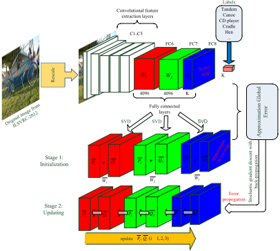
In this paper, we present a novel framework towards an "explicit" and "global" compression of CNNs, whose structure is shown in Fig. 1. Our key innovation lies in introducing a Global Error Reconstruction algorithm, which explicitly models the reconstruction error between the outputs of both the original and the compressed CNNs in a global way. In such a manner, both inter-layer and intra-layer relationships of weight parameters are jointly compressed. Meanwhile, instead of minimizing the reconstruction error between the original and approximated parameters layer-by-layer, GER directly establishes an objective function to recover the outputs of the compressed CNNs, which includes the influences of nonlinear activation functions within and across the fully connected layers.
In practice, we conduct an initial compression of the weights in the fully connected layers by an SVD-based lowrank decomposition, which can relax the constrained term of the optimization function to being trackable. Subsequently, such layer-wise, coarse compressions are further jointly optimized among layers via back propagation to minimize the global error, which is done by a novel optimization method that using the stochastic gradient descent to well solve the non-convex optimization problem.
The proposed method is evaluated on the ILSVRC2012 image classification benchmark, with testing on two widelyadopted CNNs, i.e., AlexNet [A. Krizhevsky and Hinton, 2012] and VGGNet-19 [Simonyan and Zisserman, 2014]. We have demonstrated that the proposed GER compression scheme can lead to the state-of-the-art rate-distortion 2 performance by comparing with several state-of-the-art and alternative schemes in CNN compression [M. Denil and Freitas, 2013; Y. Gong and Bourdev, 2014; X. Zhang and Sun, 2015]. The main contribution of this paper is three-fold:
- ÷ We introduce an explicit objective function to directly minimize the reconstruction error of outputs before and after network compression, which differs from the ex-
1 In this paper, we focus on the compression of the fully connected layer, as it occupies the largest proportion in the entire CNN model. For instance, above 80% storage is cost in the fully connected layers comparing to 20% in the convolutional layers of the AlexNet [A. Krizhevsky and Hinton, 2012].
2 Rate-distortion is an evaluation protocol of model compression in which the rate and distortion represent the compression rate of model and classification precision, respectively.
- isting works that indirectly minimize the difference between the original and compressed parameters.
- ÷ We globally model the inter-layer correlation during the network compression, which can address the issue of layer-wise accumulated compression error.
- ÷ We introduce an effective optimization method to solve the corresponding non-convex optimization, which firstly uses an SVD-based low-rank decomposition to relax the constrained term, and then adopts a stochastic gradient descent to learn optimal parameters.
2 Initial Compression of CNN Based on Low-rank Decomposition
2.1 Preliminaries
We define a feature matrix X = [x1↪ x2↪ · · · ↪ xn] 2 <d⇥n as the input to compress a fully-connected CNN, where d is the dimension of feature vectors, and n is the number of feature vectors which are the outputs of the last convolutional layer in the original CNN-like AlexNet [A. Krizhevsky and Hinton, 2012]. The forward propagation of the l-th layer in a compressed fully-connected CNN can be written as:
where W l ij is the element of weight matrix Wl . The vectors z↪ a 2 <nl denote the activation units before and after transformation f(·). Typically, f(·) is a non-linear transition, for instance, the rectifier linear unit (ReLU), sigmoid or tanh etc.
2.2 Layer-wise Low-rank Approximation of Linear Response
We first consider the low-rank approximation ˆWl of the original weights Wl between the l-th and l + 1-th layers. To find an approximated low-rank subspace, we minimize the reconstruction error of the neuron responses as below:
where Wl ↪ ˆWl 2 <dl+1⇥dl . With respect to the error of two linear transforms on the same input signal X, Eq. 2 can be rewritten as:
We solve Eq. 3 by Singular Vector Decomposition (SVD) [Golub and Loan, 2012], a.k.a., ˆWl = ˆUlk ˆSlk ˆVl> k , where ˆUlk 2 <dl+1⇥k and ˆVlk 2 <dl⇥k are two submatrices that correspond to the top k singular vectors in Ul and Vl . The diagonal elements in ˆSlk 2 <k⇥k correspond to the k largest Algorithm 1 Alternating optimization layer-by-layer Input: Training data points X; the output Zl between the l-th and l + 1-th layers before non-linear transformation; the input Cl between the l-th and l + 1-th layers; the restricted rank k, the maximum iterations T .
Output: The approximated low-rank matrix ˆWl .
- 1: Initialize C0 by X, the auxiliary variables Yl by Zl , and t = 1. 2: repeat
- 3: Step I: Fix Yl+1 and update ˆWl via GSVD
- 4: Step II: Fix ˆWl and updateYl+1 by analyzing each element yl+1 ij , and solve 1-dimensional optimization Eq. 9 via Eq. 10 and Eq. 11.
- 5: t := t +1;
- 6: until convergence or reach maximum iterations T
singular values in Sl , which is a diagonal matrix by running SVD over Wl . Then we obtain the decomposition of ˆWl as ˆPl ˆQl> , where ˆPl = ˆUlk ˆSl 12 k and ˆQl = ˆVlk ˆSl 12 k .
2.3 Extending to Non-Linear Responses
For non-linear transition that commonly occurs in CNNs, the result of approximated matrix is not equivalent to that of the original one. Therefore, the effect of non-linear transition should be taken into account when designing low-rank approximation of parameter matrix W. Taking the widely used ReLU transition for instance, ReLU is defined as f(·) = max(·↪ 0). To minimize the reconstruction error of ReLUlike response, we have:
where the first term ali is the non-approximated input of the lth layer (i.e. output of the l-1-th layer), and the second term ˆali approximates the input of the l-th layer. The optimization problem in Eq. 4 can be solved by a layer-wise optimization with an alternating solver. More specifically, we consider this optimization layer-to-layer in a bottom up manner: Taking Eq. 4 for example, we fix ˆali as a constant which denotes cli , and use zl+1 i instead of Wl ali in optimization. Then the optimization of each layer in Eq. 4 can be rewritten as
Unfortunately, Eq. 5 is hard to be solved due to the coexistence of the non-linearity and the low-rank constraint. To obtain a feasible solution, we relax Eq. 5 to:
where λ is a penalty parameter and yl+1 i is a set of auxiliary variables of the same size as zl+1 i . If λ ! 1, the solution to Eq. 6 will converge to the solution to Eq. 5. To solve Eq. 6, we further employ an alternating solver that alternatively fixes ¶yl+1 i ♦ and solves ˆWl , and vice versa. We detail this alternative optimization as below:
Alternating Step I: Fix ¶yl+1 i ♦ and update ˆWl , i.e.,
We rewrite Eq. 7 as a Reduced Rank Regression problem: [Gower and Dijksterhuis, 2004; Takane and Hwang, 2007],
Herek · kF is the Frobenius norm. let ¯Wl = Yl+1ClT (ClClT )-1 , Eq. 8 can be solved by the Generalized Singular Vector Decomposition (GSVD) [Takane and Jung, 2006]. i.e.,
- GSVD decomposes ¯Wl as eWl = UlSlVl . 2. The solution ˆWl to Eq. 8 is given by ˆWl = Ulk SlkVlT k , where Ulk and Vlk are the first k columns of Ul and Vl , and Slk are the k largest singular value in Sl .
- We obtain the decomposition of ˆWl = PlQl> , where Pl = Ulk Sl 12 k and Ql = Vlk Sl 12 k .
Alternating Step II: Fix ˆWl and update ¶yl+1 i ♦. Each element yl+1 ij of each vector yl+1 i is independent to any other. We then rewrite Eq. 6 as a 1-dimensional optimization process:
Algorithm 2 Global error Reconstruction for compressing CNN
Input: Training data points X; the corresponding output A after softmax function; the original weights Wl in each fullyconnected layers; the restricted rank k; the maximum number of epoch T ; the number of fully connected layers m.
Output: The low-rank matrices ˆPl and ˆQl .
- 1: Initialize ˆPl , ˆQl by low-rank decomposition of Wl ↪ l = 0↪ 1↪ · · · ↪m-1, t = 1.
- 2: repeat
- 3: Compute rˆPlJ by (17);
- 4: Compute rˆQl>J by (18);
- 5: Update ˆPl and ˆQl by SGD;
- 6: t := t +1.
- 7: until convergence or t > T.
where ¯ zl+1 ij is the j-th entry of ˆWl cli . We separately take ¯ zl+1 ij ≥ 0 and ¯ zl+1 ij 0 into account due to the restriction of ReLU. Then we derive the solution of Eq. 9:
Note that yl+1 ij = ¯ yl+1 ij if ¯ yl+1 ij have a smaller value in Eq. 9 than e yl+1 ij and otherwise yl+1 ij = e yl+1 ij . We use the gradient descent to solve the above 1-dimensional, non-linear least square problem.
The above alternating optimization is further shown in Algorithm 1. The initialization of ˆWl is given by the solution to the linear case of Eq. 3. Theoretically speaking, λ should be gradually increase to being infinity [J. Wang and Gong, 2010]. However, if λ is too large, it is difficult for the iterative solver to take effects. As a trade-off and to performmore iterations, we first increase λ to 1, and then we obtain the result ˆWl after convergence, which is adopted as the initial (coarse) compression among all the fully connected layers.
3 Cross-Layer Compression via Global Error Reconstruction
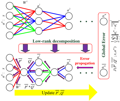
The initial compression of CNN using low-rank decomposition is to coarsely approximate ˆWl of each layer in a bottom up manner. As discussed above, the compression errors are accumulated layer-by-layer, resulting to large overall error in the output layer of CNN. To address this issue, the proposed global error reconstruction (GER) targets at jointly optimizing among layers as shown in Fig. 2.
In particular, if the original CNN model has m fully connected layers, we minimize the global reconstruction error of ReLU-like non-linear responses as follows:
where ami is the non-approximated output, and ˆam-1 i contains m- 1 weights in the hidden layers, which is written as:
To find a feasible solution, we use the solution of Eq. 4 to relax the constrain term of Eq. 12, and let Am be the matrix concatenating the vectors of ami . The objective function of Eq. 12 can be rewritten as:
where l = 0↪ 1↪ · · · ↪m- 1, and ˆAm can be written as:
In Eq. 15 ˆPl and ˆQl> are the approximate decomposition to W by solving Eq. 4. To learn the parameters ¶ˆPl ♦ and ¶ˆQl> ♦, a stochastic gradient descent algorithm is employed via back-propagation, which needs to calculate the gradient of the objective function with respect to all weights. Therefore, the error signals of the cost function in Eq. 14 is obtained via:
where ˆZl+1 = ˆPl ˆQl> · ˆAl , l = m-1↪m-2↪ · · · ↪ 0. After obtaining ˆAl+1 , we compute two gradients of objective function with respect to the parameters as follows:
where l = m - 1↪m - 2↪ · · · ↪ 0. It is worth to note that the stochastic gradient descent can reduce the accumulative errors. Algorithm 2 presents the detailed optimization algorithm for GER.
4 Experiments
To evaluate the performance of GER scheme, we conduct comprehensive experiments on ILSVRC2012 image classification benchmark. We deploy the proposed GER on two widely used CNNs (a.k.a. AlexNet [A. Krizhevsky and Hinton, 2012] and VGGNet-19 [Simonyan and Zisserman, 2014]), with comparisons to the state-of-the-art scheme proposed very recently [M. Denil and Freitas, 2013; Y. Gong and Bourdev, 2014; X. Zhang and Sun, 2015].
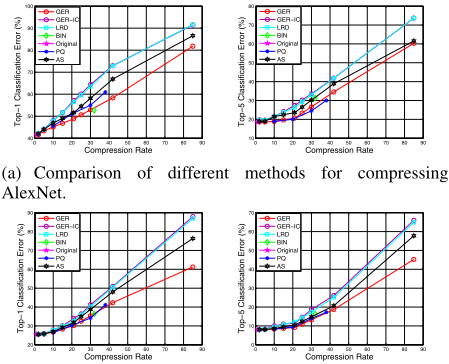
Figure 3: Comparison of methods on AlexNet and VGGNet. Values are averaged over 5 runs.
4.1 Experimental Setting
Dataset. We test the proposed GER based CNN compression on the ILSVRC2012 image classification benchmark. The dataset contains more than 1 million training images from 1,000 object classes. It also has a validation set of 50,000 images, where each object class contains 50 images. We randomly select 100,000 images (100 from each class) from the training set for training, and test on the validation set.
Implementation Details. We implement GER on two CNNs i.e., AlexNet [A. Krizhevsky and Hinton, 2012] and VGGNet-19 [Simonyan and Zisserman, 2014]. The VGGNet-19 contains 16 convolutional layers and 3 fully connected layers, and the AlexNet contains 5 convolutional layers and 3 fully connected layers. The compressed networks are trained using Caffe [Y. Jia and Darrell, 2014] and run on NVIDIA GTX TITAN X graphics card with 12GB. The learning rate starts at 0.01 and is halved every 10-epochs; the weight decay is set to 0.0005 and the momentum is set to 0.9. Baselines. We compare the proposed GER scheme with 4 state-of-the-art approaches published very recently, including PQ-based compression (PQ) [Y. Gong and Bourdev, 2014], Low-rank decomposition (LRD)[M. Denil and Freitas, 2013], Layer-wise optimization by alternating solver (AS) [X. Zhang and Sun, 2015], and Binary-based compression (BIN) [Y. Gong and Bourdev, 2014]. As for the alternative approach, we compare GER with GER-IC, which is the SVDbased initial compression based only on Sec.2.
Evaluation protocol. The classification error on the validation set was employed as the evaluation protocol. We used both the top-1 classification error and the top-5 classification error to evaluate different compression methods. Then we measure the compression performance in terms of the rate distortion, which reflects the balance between compression rate and classification error.
Rate-Distortion Comparison. We use a different rank k from 25 to 210 to achieve different compression rates. For PQ, we fix the number of centers to 256 (8 bits) and vary the segment dimension s = 1↪ 2↪ 4↪ 8. For LRD and Layer-wise optimization by alternating solver , we use the same compression criterion with GER that varies k from 25 to 210 . For BIN, which has no parameter to tune, the compression rate is fixed as 32.
| AlexNet on ILSVRC | VGGNet-19 on ILSVRC | |||||||||
|---|---|---|---|---|---|---|---|---|---|---|
| Compression rate | GER | LRD | BIN | PQ | AS | GER | LRD | BIN | PQ | AS |
| Top1 Compression rate = 16 | 47.51 | 52.63 | ⇠ | 48.83 | 49.49 | 28.63 | 30.37 | ⇠ | 28.66 | 29.59 |
| Compression rate = 32 | 53.92 | 65.01 | 52.79 | 56.45 | 59.34 | 36.52 | 41.95 | 36.37 | 35.94 | 40.29 |
| Top5 Compression rate = 16 | 20.95 | 25.24 | ⇠ | 19.33 | 23.01 | 8.74 | 11.25 | ⇠ | 8.85 | 9.47 |
| Compression rate = 32 | 27.97 | 34.67 | 31.32 | 25.93 | 31.46 | 14.11 | 18.19 | 16.29 | 14.88 | 15.91 |
Both the top-1 and top-5 classification errors are shown in Fig. 3, which show a consistent trend in rate-distortion. As for intra-layer approximation, GER-IC achieves a similar classification error to LRD. Instead, by explicitly modeling the reconstruction error in a global way, GER greatly improves rate-distortion by comparing to GER-IC. GER also performs much better than LRD and AS for compressing the fully connected layers. To explain, GER merits in its "explicit" compression, which effectively combines the initial layer-wise compression and cross-layer global compression, while LRD and AS are "implicit" compression which only consider the local intra-layer relationship. Note that PQ has achieved better performance comparing to that of LRD and AS. However, it is shown in Fig. 3 that PQ is hard to achieve high compression rate, which might be due to the limited codebook size. In contrast, GER achieves the best rate-distortion by comparing to other baselines. Finally, as discovered by Gong et al. [Y. Gong and Bourdev, 2014], the simplest BIN works well when we fixed the compression rate to 32. Therefore, The base binary quantization is also a good choice when the goal is to compress data very aggressively. However, it is hard to be adaptive when we want to control the compression rate, which in turn is one of the key advantages for our scheme. We further show that the classification error with a fixed compression rate in Tab.1 which also shows GER can achieve the best performance by comparing to other baselines especially, when implementing on VGGNet-19.
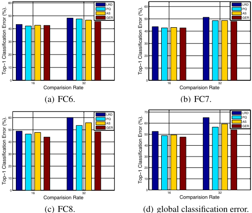
On the Single Layer Error. we further analyze the classification error by compressing each single layer while fixing the rest layers as the original uncompressed version. The results are reported in Fig. 4. We found using all the baselines to compress the first two fully connected layers (i.e. "FC6" and "FC7") does not lead to the decreasing of accuracy. In contrast, compressing the last fully connected layer leads to large classification error for all the baselines, except for the proposed GER. We explain this advantage by the fact that GER can automatically adjust the inter-layer error by tuning and refining across all layers.
5 Conclusion
In this paper, we propose to compress the convolutional neural networks to reduce the model storage by a novel Global Error Reconstruction scheme, which can facilitate emerging applications in mobile or embedding devices with limited storage. GER firstly uses an SVD-based low-rank approximations to coarsely compress the parameters in the fully connected layers. Such layer-wise initial compressions are further jointly optimized among layers in a global way via backpropagation. Unlike previous approaches that only considered recovering the internal weight parameters, GER also explicitly models the reconstruction error between the outputs of both the original and compressed CNNs, which we significantly reduces the accumulated reconstruction error caused by the nonlinear activation. We have demonstrated that the proposed GER scheme can lead to state-of-the-art ratedistortion performance by comparing to several very recent schemes in CNN compression [M. Denil and Freitas, 2013; Y. Gong and Bourdev, 2014; X. Zhang and Sun, 2015]. In our future work, we would extend and evaluate our compression scheme from the fully connected layer to the convolutional layer, and at the same time, further accelerate computation of convolutional layers.
Acknowledgments
This work is supported by the Special Fund for Earthquake Research in the Public Interest No.201508025, the Nature Science Foundation of China (No. 61402388, No. 61422210 and No. 61373076), the Fundamental Research Funds for the Central Universities (No. 20720150080 and No.2013121026), and the CCF-Tencent Open Research Fund.
@inproceedings{ijcai2016p251,
  title     = {Towards Convolutional Neural Networks Compression via Global Error Reconstruction},
  author    = {Lin, Shaohui and Ji, Rongrong and Guo, Xiaowei and Li, Xuelong},
  booktitle = {Proceedings of the Twenty-Fifth International Joint Conference on
               Artificial Intelligence, {IJCAI-16}},
  publisher = {AAAI Press / International Joint Conferences on Artificial Intelligence},
  editor    = {Subbarao Kambhampati},
  pages     = {1753--1758},
  year      = {2016},
  month     = {7},
  url       = {https://ijcai.org/proceedings/2016/251},
}
TY - CPAPER TI - Towards Convolutional Neural Networks Compression via Global Error Reconstruction AU - Lin, Shaohui AU - Ji, Rongrong AU - Guo, Xiaowei AU - Li, Xuelong T2 - Proceedings of the Twenty-Fifth International Joint Conference on Artificial Intelligence, IJCAI-16 PB - AAAI Press / International Joint Conferences on Artificial Intelligence PY - 2016 SP - 1753 EP - 1758 UR - https://ijcai.org/proceedings/2016/251 ER -Copied
Machine-readable versions of this paper, for tools and AI agents:





