A Decision Procedure for a Fragment of Linear Time Mu-Calculus

1 Introduction

Linear Temporal Logic (LTL) is a convenient formalism for specifying and verifying properties of reactive systems [Pnueli, 1977]. Also, due to its simplicity, it has been extensively used in planning for temporally extended goals [Bacchus and Kabanza, 1998; De Giacomo and Vardi, 1999; Calvanese et al., 2002; Kabanza and Thi´ebaux, 2005; Baier and McIlraith, 2006; Patrizi et al., 2011]. However, restricted by its expressiveness, LTL cannot be used to specify relatively complex goals. Therefore, extensions of LTL [De Giacomo and Vardi, 2013; 2015] have been studied in order to make it more powerful. Unfortunately, these extensions consider only finite LTL rather than standard LTL over infinite traces.

To this end, we investigate a fragment, called Gθ, of linear time θ-calculus (⌫TL) over infinite traces [Barringer et al., 1986] as a high-level goal specification language. ⌫TL is an extension of LTL with least and greatest fixpoint operators whose expressive power is !-regular [Emerson and Clarke, 1980]. Fixpoints not only nicely capture the nonterminating behaviors of intelligent systems, but also allow us to express a much wider range of temporally extended goals than LTL does. However, the current best time complexity for the decision problem of ⌫TL is 2O(♣φ♣2 log ♣φ♣) [Kaivola, 1995; Bradfield et al., 1996; Dax et al., 2006], which prevents ⌫TL

⇤Corresponding authors. All authors are joint first authors.

from being used directly as goal formulas for planning. Given a formula φ, the logic Gθ we present in this paper stipulates, for each least fixpoint subformula F of φ and each formula of the form φ1 ^ φ2 in the closure of φ, that F appears at most in one conjunct of φ1 ^ φ2. Despite this restriction, Gθ is still very expressive. Consider the following goal: "a sweeping robot must clean a house on every Monday (whether it cleans the house on other days is not cared about)". Obviously, such a goal is not expressible in LTL. However, it can be easily specified by a simple greatest fixpoint formula ⌫X▷(pmon ^©©©©©©©X) of Gθ.

In this paper, we focus on the satisfiability problem of Gθ. Motivated by the idea of formula progression [Bacchus and Kabanza, 1998], we define Goal Progression Form (GPF) for Gθ formulas and prove that every closed formula can be transformed into this form. GPF decomposes a formula into the present and future parts. The present part is the conjunction of atomic propositions or their negations while the future part is the conjunction of elements in the closure of a given formula. Additionally, based on GPF, we introduce the notion of Goal Progression Form Graph (GPG) which can be used to describe models of a formula. In a GPG, an edge may be associated with a mark which is a subset of variables occurring in the formula and utilized to keep track of the infinite unfolding problem for least fixpoints. Further, we present a decision procedure for checking satisfiability of Gθ formulas based on GPG. It is achieved, with the help of marks, by searching for a ⌫-path in a GPG on which no least fixpoint unfolds itself infinitely. We show that the time complexity of the proposed decision procedure is 2O(♣φ♣) , which is equivalent to that of LTL [Sistla and Clarke, 1985]. This makes Gθ useful in temporal planning: with Gθ, more goals can be specified than utilizing LTL while the complexity keeps the same with LTL.

GPGs are very useful for generating plans for Gθ goals by exploiting ⌫-paths. Moreover, following the decision procedure mentioned above, we can easily obtain a GPG-based model checking approach for Gθ which can be further applied to dealing with different kinds of planning problems.

2 Preliminaries

Let P be a set of atomic propositions, and V a set of variables. ⌫TL formulas are constructed based on the following syntax:

where p ranges over P and X over V.

We use σ to denote either θ or ⌫, and ˙p to denote either p or ≻p. An occurrence of a variable X in a formula is called free if it does not lie in the scope of σX; it is called bound otherwise. A formula is called closed if it contains no free variables. We write φ[φ0 ◁Y ] for the result of simultaneously substituting φ0 for all free occurrences of the variable Y in φ. For each variable X in a formula, we assume that X is bound at most once. Thus, it can be seen that all formulas constructed by the syntax above are in positive normal form [Kozen, 1983], i.e. negations can be applied only to atomic propositions and each variable occurring in a formula is bound at most once. Then, for each bound variable X in a formula φ, there exists a unique fixpoint subformula σX▷' of φ identified by X. A θ-variable (resp. ⌫-variable) in φ is a variable which identifies a formula of the form θX▷' (resp. ⌫X▷').

For two formulas σX▷φ and σY▷φ0 where σY▷φ0 is a subformula of σX▷φ, we say Y depends on X, denoted by X C Y , iff X occurs free in φ0 . The dependency relationship among the variables in a formula is transitive.

A formula is guarded if, for each bound variable X in that formula, every occurrence of X is in the scope of a next (©) operator. Every formula can be transformed into an equivalent one in guarded form with an exponential increase in the size of the formula in the worst case [Bruse et al., 2015].

⌫TL formulas are interpreted over linear time structures. A linear time structure over P is a function K: N ! 2P where N denotes the set of natural numbers. The semantics of ⌫TL formulas, relative to K and an environment e : V ! 2N , is defined as follows:

where e[X 7! W] is the environment e0 agreeing with e except for e0 (X) = W. e is used to evaluate free variables and can be dropped when φ is closed.

For a given formula φ, we say φ is true at state i of a linear time structure K, denoted by K↪ i ♣= φ, iff i 2 kφkKe . We say φ is valid, denoted by ♣= φ, iff K↪ j ♣= φ for all linear time structures K and all states j of K; φ is satisfiable iff there exists a linear time structure K and a state j of K such that K↪ j ♣= φ.

Let Ord denote the class of ordinals. Approximants of fixpoint formulas are defined inductively by: θ0X▷φ = ?, ⌫ 0X▷φ = >, σ↵+1X▷φ = φ[σ↵X▷φ◁X], θλX▷φ = W↵<λ θ↵X▷φ and ⌫ λX▷φ = V↵<λ ⌫ ↵X▷φ where ↵↪ λ 2 Ord. In particular, λ is a limit ordinal. The following lemma [Tarski, 1955] is a standard result about approximants.

Lemma 1 ([Tarski, 1955]) For a linear time structure K, we say K↪ 0 ♣= ⌫X▷φ iff 8↵ 2 Ord, K↪ 0 ♣= ⌫ ↵X▷φ; and K↪ 0 ♣= θY▷φ iff 9↵ 2 Ord, K↪ 0 ♣= θ↵Y▷φ.

The closure CL(φ) of a formula φ, based on [Fischer and Ladner, 1979], is the least set of formulas such that: (1) φ↪ true 2 CL(φ); (2) if ' _ or ' ^ 2 CL(φ), then '↪ 2 CL(φ); (3) if ©' 2 CL(φ), then ' 2 CL(φ); (4) if σX▷' 2 CL(φ), then '[σX▷'◁X] 2 CL(φ). It has been proved that the size of CL(φ) is linear in the size of φ (denoted by ♣φ♣) [Fischer and Ladner, 1979].

Given a formula φ, we call it a Gθ formula iff for each least fixpoint subformula θX▷' of φ we are focusing on and each φ1 ^ φ2 2 CL(φ), θX▷' appears at most in one φi (i 2 ¶1↪ 2♦). For example, ⌫X▷θY▷(©Y _ p ^ ©X) and θX▷(q _ p ^©X) ^ ⌫Y▷(r ^©©Y ) are Gθ formulas while ⌫X▷(θY▷(p _ ©Y ) ^ ©X) and θX▷(p _ ©X ^ © © X) are not. The syntax of Gθ enables us to trace conveniently the infinite unfolding problem for least fixpoints and provide efficient decision procedures.

Gθ can be employed to specify a wide variety of properties. Currently, there already exists a fragment of modal θcalculus [Kozen, 1983], called deterministic θ-calculus (Dθ), which has been used in motion planning [Karaman and Frazzoli, 2009]. The syntax of Dθ is defined as follows:

Compared with modal θ-calculus, Dθ allows only the existential next-state operator ⌃. Moreover, for the boolean connective ^, at least one conjunct is a proposition. Despite its succinct syntax, Dθ is able to specify all !-regular properties. However, due to the strict restriction on the boolean connective ^, many properties cannot be directly expressed in Dθ. We can employ Gθ to overcome this weakness. For instance, the Gθ formula θX▷(q _ p ^©X) ^ ⌫Y▷(r ^©©Y ) cannot be intuitively represented as a formula in Dθ. Since the restriction on the boolean connective ^ for Gθ is strictly weaker than that for Dθ, Gθ will be no less in expressive power than Dθ.

From now on, we confine ourselves to Gθ formulas in guarded form with no _ appearing as the main operator under each next (©) operator. This can be easily achieved by pushing next (©) operators inwards using the equivalence ©(φ1 _ φ2) ⌘ ©φ1 _ ©φ2.

3 GPF of Gθ Formulas

In this section, we define GPF of Gθ formulas and prove that every closed formula can be transformed into this form.

Definition 1 Let φ be a closed formula, Pφ the set of atomic propositions appearing in φ. GPF of φ is defined by: φ ⌘ Wni=1 (φpi ^ ©φfi ), where φpi ⌘ Vn1 h=1 ˙ qih, qih 2 Pφ for each h, and φfi ⌘ Vn2 m=1 φim, φim 2 CL(φ) for each m.

Intuitively, in a GPF, φpi represents the present part while φfi represents the future one.

Theorem 2 Every closed formula ' can be transformed into GPF.

Proof. Let Conj( ) represent the set of all conjuncts in . The proof proceeds by induction on the structure of '.

÷ Base case:

• ' is p (or ≻p): p (or ≻p) can be written as: p ⌘ p ^ ©true (or ≻p ⌘ ≻p ^ ©true). Therefore, ' can be transformed into GPF in these two cases.

÷ Induction:

• ' is ©φ: ©φ can be written as: ©φ ⌘ Wi (true^©φi). For each φc 2 Conj(φi), we have φc 2 CL(') since φ 2 CL('). Hence, ' can be transformed into GPF in this case.
• ' is φ1_φ2: by induction hypothesis, both φ1 and φ2 can be transformed into GPF: φ1 ⌘ Wni=1 (φ1pi ^©φ1fi ), φ2 ⌘ Wmj=1 (φ2pj ^©φ2fj ) where φ1c 2 Conj(φ1fi ) and φ1c 2 CL(φ1), φ2c 2 Conj(φ2fj ) and φ2c 2 CL(φ2), for each i and j. Then, we have ' ⌘ φ1_φ2 ⌘ Wni=1 (φ1pi ^ ©φ1fi ) _ Wmj=1 (φ2pj ^ ©φ2fj ). Since φ1 _ φ2 2 CL('), we have φ1↪ φ2 2 CL('). For each φ1c 2 Conj(φ1fi ), by induction hypothesis, we have φ1c 2 CL(φ1). Therefore, φ1c 2 CL('). Similarly, we can obtain that each φ2c 2 CL('). Thus, ' can be transformed into GPF in this case.
• ' is φ1^φ2: by induction hypothesis, both φ1 and φ2 can be transformed into GPF: φ1 ⌘ Wni=1 (φ1pi ^©φ1fi ), φ2 ⌘ Wmj=1 (φ2pj ^©φ2fj ) where φ1c 2 Conj(φ1fi ) and φ1c 2 CL(φ1), φ2c 2 Conj(φ2fj ) and φ2c 2 CL(φ2), for each i and j. Then ' can be further converted into: ' ⌘ φ1 ^ φ2 ⌘ (Wni=1 (φ1pi ^©φ1fi )) ^ (Wmj=1 (φ2pj ^ ©φ2fj )) ⌘ Wni=1 Wmj=1 (φ1pi ^ φ2pj ^ ©(φ1fi ^ φ2fj )). Since φ1 ^ φ2 2 CL('), we have φ1↪ φ2 2 CL('). For each φ1c 2 Conj(φ1fi ), by induction hypothesis, we have φ1c 2 CL(φ1). Hence, φ1c 2 CL('). Similarly, we can obtain that each φ2c 2 CL('). Therefore, all conjuncts behind the next (©) operators in ' belong to CL(') and ' can be transformed into GPF in this case.
• ' is θX▷φ: to transform θX▷φ into GPF, we first need to unfold it using the equivalence θX▷φ ⌘ φ[θX▷φ◁X]. That is to say, we can treat the free variable X occurring in φ as an atomic proposition when transforming φ into GPF since X will finally be replaced by θX▷φ. As a result, by induction hypothesis, φ can be transformed into GPF: φ ⌘ Wni=1 (φpi ^ ©φfi ). For each φc 2 Conj(φfi ), by induction hypothesis, we have φc 2 CL(φ). Further, by substituting θX▷φ for all the free occurrences of X in φ, we have that ' ⌘ φ[θX▷φ◁X] ⌘ Wni=1 (φpi ^ ©φfi [θX▷φ◁X]). Since φc 2 CL(φ) for each φc, we can easily obtain that φc[θX▷φ◁X] 2 CL(φ[θX▷φ◁X]) after the substitution. Since φ[θX▷φ◁X] 2 CL('), we have φc[θX▷φ◁X] 2 CL('). Therefore, ' can be transformed into GPF in this case.
• ' is ⌫X▷φ: this case can be proved similarly to the case when ' is θX▷φ. ⇤

Following Theorem 2, we present algorithm GPFTr in the following for transforming a closed formula φ into GPF.

GPFTr uses the function AND to deal with the boolean connective ^. It can be seen that the inputs, and ', for AND are both in GPF. Suppose is of the form Wi ( i ^ © 0i )

Algorithm 1 GPFTr(φ)

• 1: case
• 3: φ is false: return false
• 2: φ is true: return true ^©true
• 5: φ is φp ^©': return Wi (φp ^©'i)
• 4: φ is φp where φp ⌘ Vnh=1 ˙ qh: return φp ^©true
• 8: φ is φ1 ^ φ2: return AND(GPFTr(φ1), GPFTr(φ2))
• 6: φ is ©': return Wi (true ^©'i) 7: φ is φ1 _ φ2: return GPFTr(φ1) _ GPFTr(φ2)
• 9: φ is σX▷': return GPFTr('[σX▷'◁X])

10: end case

while ' of the form Wj ('j ^ ©'0j ). AND finally returns Wi Wj ( i ^'j ^©( 0i ^'0j )).

Theorem 3 Transforming a formula φ into GPF by algorithm GPFTr can be completed in 2O(♣φ♣) .

Proof. The proof proceeds by induction on the structure of φ.

÷ Base case:

• φ is true, false, φp, φp ^©' (where φp is of the form Vnh=1 ˙ qh), or ©': the theorem holds obviously in these cases.
• φ is φ1 _ φ2: by induction hypothesis, GPFTr(φ1) and GPFTr(φ2) can be done in 2O(♣φ1♣) and 2O(♣φ2♣) , respectively. Therefore, GPFTr(φ) can be finished in 2O(♣φ1♣) + 2O(♣φ2♣) , namely 2O(♣φ♣) .

÷ Induction:

• φ = φ1 ^ φ2: by induction hypothesis, GPFTr(φ1) and GPFTr(φ2) can be completed in 2O(♣φ1♣) and 2O(♣φ2♣) , respectively. After the GPF transformation, the number of disjuncts in φ1 (resp. φ2) is bounded by 2O(♣φ1♣) (resp. 2O(♣φ2♣) ). Hence, the function AND can be accomplished in 2O(♣φ1♣+♣φ2♣) . It follows that GPFTr(φ) can be done in 2O(♣φ1♣) + 2O(♣φ2♣) + 2O(♣φ1♣+♣φ2♣) , namely 2O(♣φ♣) .
• φ = σX▷': regarding X as an atomic proposition, ' can be transformed into GPF by algorithm GPFTr, which can be accomplished, by induction hypothesis, in 2O(♣'♣) . Subsequently, by substituting σX▷' for all free occurrences of X in ', we have that '[σX▷'◁X] can be transformed into GPF by algorithm GPFTr in 2O(♣'♣) . Therefore, GPFTr(σX▷') can be done in 2O(♣φ♣) . ⇤

4 Goal Progression FormGraph

The GPG, Gφ, of a formula φ is a tuple (Nφ↪ Eφ↪ n0) where Nφ is a set of nodes, Eφ a set of directed edges, and n0 the root node. Each node in Nφ is specified by the conjunction of formulas in CL(φ) while each edge in Eφ is identified by a triple (φ0↪ φe↪ φ1), where φ0, φ1 2 Nφ and φe is the label of the edge from φ0 to φ1. An edge may be associated with a mark which is a subset of variables occurring in φ.

Definition 2 Given a closed formula φ. Nφ and Eφ are inductively defined by: (1) n0 = φ 2 Nφ; (2) for all ' 2 Nφ∩¶false♦, if ' ⌘ Wki=1 ('pi ^©'fi ), then 'fi 2 Nφ, ('↪ 'pi ↪ 'fi ) 2 Eφ for each i (1  i  k).

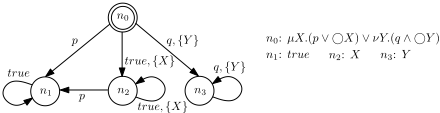
In a GPG, the root node is denoted by a double circle while each of other nodes by a single circle. Each edge is denoted by a directed arc with a label and also possibly a mark that connects two nodes. To simplify notations, we usually use variables to represent the corresponding fixpoint formulas occurring in a node. An example of GPG for formula θX▷(p _©X) _ ⌫Y▷(q ^©Y ) is depicted in Figure 1. There are four nodes in the GPG where n0 is the root node. (n0↪ q↪ n3) is an edge with the label being q and the mark being ¶Y ♦ while (n0↪ p↪ n1) is an edge with the label being p and no mark.

true↪ ¶X♦

Figure 1: An example of GPG

A path ⇧ in a GPG is an infinitely alternate sequence of nodes and edges departing from the root node. Let Atom(Vmi=1 ˙ qi) denote the set of atomic propositions or their negations appearing in formula Vmi=1 ˙ qi. Given a path ⇧ = φ0↪ φe0↪ φ1↪ φe1↪ ▷ ▷ ▷ in a GPG, we can obtain its corresponding linear time structure Atom(φe0)↪ Atom(φe1)↪ ▷ ▷ ▷. For example, in Figure 1, the path n0↪ true↪ n2↪ p↪ (n1↪ true)! corresponds to the linear time structure ¶true♦¶p♦¶true♦! .

From Figure 1 we can see that there may exist a path in a GPG, e.g. n0↪ true↪ (n2↪ true)! , which arises from the infinite unfolding of a least fixpoint. Thus, marks are essential in a GPG to keep track of the infinite unfolding problem for least fixpoints when constructing the GPG.

Definition 3 Given a GPG Gφ and a node φm 2 Nφ where φm ⌘ Wki=1 (φpi ^ ©φfi ). The mark of an edge (φm↪ φpi ↪ φfi ) (1  i  k) is a set of variables Mv such that for each X 2 Mv, its corresponding fixpoint formula σX▷φX appears as a subformula of φfi and has been unfolded by itself in the GPF transformation process.

When transforming a formula into GPF, the occurrence of a fixpoint formula σX▷φX in the future part may be caused by the unfolding of either (I) itself, or (II) another fixpoint formula. For example, as shown in Figure 2, when the node n0 is transformed into GPF: n0 ⌘ true ^ ©n1, the occurrence of ⌫Y▷(p ^ ©Y ) in n1 is due to the unfolding of θX▷©(©⌫Y▷(p^©Y )^X), hence Y does not exist in the mark of the edge (n0↪ true↪ n1).

Note that the cases I and II above may occur simultaneously for a greatest fixpoint formula ⌫Z▷φZ, we will add Z to the corresponding mark in such a situation, e.g. the occurrence of Y in the mark of the edge (n2↪ p↪ n2) in Figure 2. However, for a least fixpoint formula, the cases I and II

cannot happen simultaneously due to the syntactic restriction of Gθ. Actually, this restriction makes, for a given formula φ, each θX▷' 2 CL(φ) occur at most in one conjunct of each node in Gφ. This further facilitates the tracing of the infinite unfolding problem for least fixpoints.

Given a closed formula φ, the whole process of constructing Gφ is presented in Algorithm 2.

Algorithm 2 GPGCON(φ)

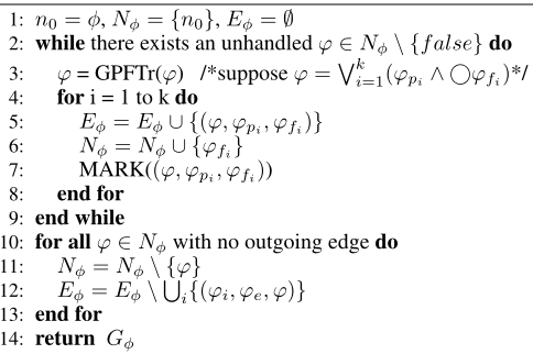
The algorithm repeatedly converts an unhandled formula ' 2 Nφ into GPF and then adds the corresponding nodes and edges to Nφ and Eφ, respectively, until all formulas in Nφ have been handled. Function MARK is utilized to mark an edge with a subset of variables occurring in φ by distinguishing appropriate fixpoint formulas from all fixpoint formulas contained in the future part of a certain GPF. Given an edge ('↪ 'pi ↪ 'fi ), MARK checks each conjunct 'c of 'fi . If 'c is of the form©nσX▷'X (n ≥ 0) and σX▷'X has been unfolded by itself in the GPF transformation process, X will be added to the mark of the edge. Here ©n represents the consecutive occurrence of next (©) operators for n times. Additionally, throughout the construction of Gφ, a false node (e.g. q ^ ≻q) may be generated which corresponds to an inconsistent subset of CL(φ). Such kind of nodes have no successor and are redundant. We use the for loop in Line 10 of the algorithm to remove these nodes and the relative edges.

In the GPG Gφ of a formula φ, since each node in Nφ is the conjunction of formulas in CL(φ), the following corollary is easily obtained.

Corollary 4 For any closed formula φ, both the number of nodes and the number of edges in Gφ are bounded by 2O(♣φ♣) .

Theorem 5 Constructing the GPG of a formula φ by algorithm GPGCON can be done in 2O(♣φ♣) .

Proof. By Corollary 4, the number of iterations of the while loop is bounded by 2O(♣φ♣) . In each iteration, algorithm GPFTr is called first, which can be done in 2O(♣φ♣) by Theorem 3. Subsequently, after the GPF transformation, we have that the number of iterations of the for loop in Line 4 is bounded by 2O(♣φ♣) . Function MARK checks if a fixpoint formula, which has been unfolded by itself in a GPF transformation process, exists in the future part of the GPF and can be completed in O(♣φ♣). Therefore, the while loop can be finished in 2O(♣φ♣) . Further, it is obvious that eliminating redundant nodes and the relative edges can be finished in 2O(♣φ♣) . Consequently, GPGCON can be done in 2O(♣φ♣) . ⇤

5 ADecision Procedure Based on GPG

In this section we show how to find a model for a given formula φ from Gφ. According to the theory of eventually periodic models [Banieqbal and Barringer, 1989], we restrict ourselves here only to the paths ending with loops in Gφ. Let ⇧ be a path in Gφ, for convenience, we use LES(⇧) to denote the set of edges appearing in the loop part of ⇧, Mark(e) the mark of an edge e, and LMS(⇧) the set of all the θ-variables occurring in each Mark(el) where el 2 LES(⇧).

In the following, we present the notion of ⌫-paths which will play a vital role in obtaining the GPG-based decision procedure for Gθ.

Definition 4 Given a GPG Gφ and a path ⇧ in Gφ. We call ⇧ a ⌫-path iff for each X 2 LMS(⇧), an edge e 2 LES(⇧) can be found such that X ◁2 Mark(e) and there exists no X0 2 Mark(e) where X C X0 .

We consider the following two paths in Figure 1 to show what a ⌫-path is: (1) ⇧1: n0↪ q↪ (n3↪ q)! . ⇧1 is a ⌫-path since LMS(⇧1) = ;; (2) ⇧2: n0↪ true↪ (n2↪ true)! . We have that LES(⇧2) = ¶(n2↪ true↪ n2)♦ and LMS(⇧2) = ¶X♦. For the only θ-variable X 2 LMS(⇧2), we cannot find an edge from LES(⇧2) whose mark does not contain X. Therefore, ⇧2 is not a ⌫-path.

Regarding the notion of ⌫-paths, the following theorem is formalized.

Theorem 6 A closed formula φ is satisfiable iff a ⌫-path can be found in Gφ.

Proof. ()) Suppose φ is satisfiable and no ⌫-path exists in Gφ. In this case, for any path ⇧1 = φ0↪ φe0↪ φ1↪ φe1↪ ▷ ▷ ▷ ↪ (φk↪ φek↪ φk+1↪ φe(k+1)↪ ▷ ▷ ▷ ↪ φl↪ φel)! in Gφ, there exists at least one X 2 LMS(⇧1) such that for each edge e1 2 LES(⇧1), either X 2 Mark(e1) or X0 2 Mark(e1), where X C X0 . As a result, we can obtain the following sequence of variables X according to the sequence of marks in the loop part of ⇧1: X1↪X2↪X3↪ ▷ ▷ ▷ ↪Xl-k+1, where each Xi 2 Mark((φi+k-1↪ φe(i+k-1)↪ φi+k)) (1  i  l - k + 1) is either X itself or a variable depending on X. Let φXi denote the conjunct in φi+k corresponding to Xi, then X determines a sequence of formulas ΦX: φX1 ↪ φX2 ↪ φX3 ↪ ▷ ▷ ▷ ↪ φXl-k+1 . For each variable Xj on X that depends on X, we have that θX▷φX appears as a subformula of φXj , where θX▷φX 2 CL(φ) represents the fixpoint formula corresponding to X. Suppose ⇧1 characterizes a model K. There must exist a state t1 of K where θX▷φX can be satisfied. By Lemma 1, there exists an ordinal m such that K↪ t1 ♣= θmX▷φX. Pushing this satisfaction further down the sequence ΦX, we will eventually reach a state t2 of K such that K↪ t2 ♣= θ0X▷φX, which is impossible. Therefore, we can see that ⇧1 does not characterize a model of φ. This contradicts the premise that φ is satisfiable. Therefore, if φ is satisfiable, there exists at least one ⌫-path in Gφ.

(() Let ⇧2 = φ0↪ φe0↪ φ1↪ φe1↪ ▷ ▷ ▷ ↪ (φk↪ φek↪ φk+1↪ φe(k+1)↪ ▷ ▷ ▷ ↪ φl↪ φel)! be a ⌫-path in Gφ. When LMS(⇧2) is empty, the infinite unfolding problem for least fixpoints will not be involved on ⇧2. Consequently, ⇧2 characterizes a model of φ in this case.

When LMS(⇧2) is not empty, we have that for each Y 2 LMS(⇧2), an edge e2 2 LES(⇧2) can be found such that Y ◁2 Mark(e2) and there exists no Y 0 2 Mark(e2) where Y CY 0 . Subsequently, we can obtain the following sequence of variables Y according to the sequence of marks in the loop part of ⇧2: Y1↪ Y2↪ ▷ ▷ ▷ ↪ Yj↪ Yj+1↪ ▷ ▷ ▷ ↪ Yl-k+1, where each Yi 2 Mark((φi+k-1↪ φe(i+k-1)↪ φi+k)) (1  i  l -k +1), and Yj is neither Y nor a variable depending on Y while any other variable on Y is the opposite. Let φYi denote the conjunct in φi+k corresponding to Yi, then Y determines a sequence of formulas ΦY : φY1 ↪ φY2 ↪ φY3 ↪ ▷ ▷ ▷ ↪ φYl-k+1 . Further, we have that θY▷φY does not appear as a subformula of φYj , where θY▷φY 2 CL(φ) represents the fixpoint formula corresponding to Y . Similarly, we can obtain that ⇧2 characterizes a model of φ using the notion of approximants. It follows that when there exists a ⌫-path in Gφ, φ is satisfiable. ⇤

Consequently, we reduce the satisfiability problem of a formula to a ⌫-path searching problem from its GPG. In the following, we present algorithm NuSearch used to find a ⌫-path from a GPG.

Algorithm 3 NuSearch(n0)

1: NS.push back(n0) 2: for each edge e in Gφ do 3: if src[e] = n0 and visit[e] = 0 then 4: ES.push back(e) 5: visit[e] = 1 6: if LOOP(tgt[e], pos) then 7: TES.assign(ES.begin() + pos, ES.end()) 8: if TES corresponds to a ⌫-path then 9: return satisfiable 10: end if 11: ES.pop back() 12: else 13: NuSearch(tgt[e]) 14: end if 15: end if 16: end for 17: if ES.size() > 0 then 18: ES.pop back() 19: end if 20: NS.pop back()

Given a GPG Gφ, the algorithm first takes the root node n0 of Gφ as input and tries to build a ⌫-path. Two global variables, ES and NS, are used in the algorithm. ES is a vector which stores the sequence of edges aiming to construct a path ending with a loop. NS is also a vector storing the sequence of nodes corresponding to ES. In addition, src[] and tgt[] are employed to obtain the source and target nodes of an edge, respectively. visit[e] = 1 (or. 0) indicates that an edge e has (or. has not) been visited. For each edge e in Gφ, visit[e] is initialized to 0. LOOP is a simple boolean function which determines whether a node u exists in NS and obtains, if so, the position pos of u in NS.

In algorithm NuSearch, n0 is added to NS first. After that, for each unvisited edge e in Gφ whose source node is n0, the algorithm adds it to ES and assigns visit[e] to 1. Then, it determines whether tgt[e] exists in NS by means of function LOOP. If the output of LOOP is true, there exists a loop in ES and we use TES to store the loop of ES. Further, if TES corresponds to a ⌫-path, the given formula is satisfiable and the algorithm terminates; otherwise, the last edge in ES is removed and a new for loop begins in order to search for another unvisited edge from Gφ whose source node is n0 to establish a new path. In case the output of LOOP is false, which means the current ES cannot construct a path ending with a loop, the algorithm calls itself and tries to build new paths from the node tgt[e]. If the conditional statement in Line 3 is never satisfied, i.e. any edge in Gφ with n0 being its source node has been visited, n0 is removed from NS. Note that if the size of ES is greater than 0 when the for loop terminates, we need to remove the last edge in ES generated by the next level of recursion.

Theorem 7 For the GPG Gφ of a closed formula φ, algorithm NuSearch can be completed in 2O(♣φ♣) .

Proof. By Corollary 4, we have that both the number of nodes ♣Nφ♣ and the number of edges ♣Eφ♣ in Gφ are bounded by 2O(♣φ♣) . Since each edge in Gφ is handled exactly once, the total number of recursive calls for NuSearch is bounded by 2O(♣φ♣) . Moreover, the number of iterations of the for loop is also bounded by 2O(♣φ♣) . Subsequently, function LOOP checks whether a node exists in NS, which can apparently be done in 2O(♣φ♣) . Further, since the size of TES is in 2O(♣φ♣) , by maintaining, for each θ-variable X occurring in φ, a list of variables depending on X, we can determine whether TES corresponds to a ⌫-path in 2O(♣φ♣) . Therefore, algorithm NuSearch can be completed in 2O(♣φ♣) . ⇤

As a consequence of Theorems 5 and 7, we obtain the following theorem.

Theorem 8 For a given closed formula φ, the GPG-based decision procedure can be done in 2O(♣φ♣) .

6 RelatedWork

GPG is a useful formalism for describing the models satisfying a formula. Therefore, it can be employed to generate plans for Gθ goals. More precisely, it is ⌫-paths in a GPG that characterize such plans. Representing Gθ goals as GPGs is similar to the compilation approaches [Rintanen, 2000; Cresswell and Coddington, 2004; Kabanza and Thi´ebaux, 2005; Edelkamp, 2006; Baier and McIlraith, 2006; Patrizi et al., 2011] to planning for LTL goals which exploit the relationship between LTL and finite-state automata (FSA). The compilation approaches are particularly useful when there exists no search control knowledge. Recently, a novel method [Torres and Baier, 2015] to compile away finite LTL goals running in polynomial time is proposed. The method exploits alternating automata instead of FSA. However, all the abovementioned methods consider LTL goals, which are less expressive than Gθ goals presented in this paper. In addition, although LTL has been extended in [De Giacomo and Vardi, 2013; 2015] in order to express a wider variety of goals, these extensions, unfortunately, consider only LTL over finite traces, which can be more easily handled than standard LTL over infinite traces. In contrast, our logic Gθ focuses on infinite traces.

The decision problems of ⌫TL have been extensively studied. In [Vardi, 1988], Vardi first adapts the classical automata theoretic decision procedure for modal θ-calculus [Streett and Emerson, 1984] to ⌫TL with past operators, yielding an algorithm running in 2O(♣φ♣4 ) . Later, Banieqbal and Barringer [Banieqbal and Barringer, 1989] demonstrate that the satisfiability problem of a formula can be reduced to a good path searching problem from a graph. This method is equivalent in time complexity to Vardi's but runs in exponential space. In [Stirling and Walker, 1990], the first tableau characterization for ⌫TL's decision problems is presented without mentioning complexity issues. After that, based on the work in [Kaivola, 1995], the tableau system is improved by simplifying the success conditions for a tableau [Bradfield et al., 1996]. The algorithm obtained runs in 2O(♣φ♣2 log ♣φ♣) . Further, a proof system for checking validity of ⌫TL formulas is proposed in [Dax et al., 2006] which runs in 2O(♣φ♣2 log ♣φ♣) and has been implemented in OCAML. However, the complexities of these decision procedures are too high, which hinders the use of ⌫TL goals in planning. Therefore, we focus on an expressive fragment Gθ of ⌫TL in this paper and provide a better GPG-based decision procedure running in 2O(♣φ♣) . This makes Gθ a compelling goal specification language.

It is worth pointing out that the idea of breaking a formula into the present and future parts has also been considered in [Duan et al., 2008; Duan and Tian, 2014; Duan et al., 2016] to solve the decidability problem of Propositional Projection Temporal Logic (PPTL).

7 Conclusion

In this paper, we have investigated an expressive fragment Gθ of ⌫TL and presented GPF and GPG for Gθ formulas. Also, we have proposed a simple GPG-based decision procedure for checking satisfiability of Gθ formulas running in 2O(♣φ♣) , which makes Gθ a compelling alternative for specifying a richer class of goals in planning compared with LTL.

In the future, we are going to implement the proposed decision procedure. We also plan to develop a GPG-based model checker to solve different kinds of planning problems.

Acknowledgments

The authors would like to thank all the anonymous reviewers for their valuable comments on this paper. This research is supported by the National Natural Science Foundation of China Grant Nos. 61133001, 61322202, 61420106004, and 91418201.