
Unsupervised Machine Condition Monitoring Using Segmental Hidden Markov Models
Proceedings of the Twenty-Fourth International Joint Conference on Artificial Intelligence. Special Track on Machine Learning. Pages 4009-4015.
© 2015 International Joint Conferences on Artificial Intelligence
Abstract
The task of machine condition monitoring is to detect machine failures at an early stage such that maintenance can be carried out in a timely manner. Most existing techniques are supervised approaches: they require user annotated training data to learn normal and faulty behaviors of a machine. However, such supervision can be difficult to acquire. In contrast, unsupervised methods don't need much human involvement, however, they face another challenge: how to model the generative (observation) process of sensor signals. We propose an unsupervised approach based on segmental hidden Markov models. Our method has a unifying observation model integrating three pieces of information that are complementary to each other. First, we model the signal as an explicit function over time, which describes its possible non-stationary trending patterns. Second, the stationary part of the signal is fit by an autoregressive model. Third, we introduce contextual information to break down the signal complexity such that the signal is modeled separately under different conditions. The advantages of the proposed model are demonstrated by tests on gas turbine, truck and honeybee datasets.
- [Antoniadou et al., 2015] I. Antoniadou, N. Dervilis, E. Pap- atheou, A. E. Maguire, and K. Worden. Aspects of struc- tural health and condition monitoring of offshore wind turbines. Philosophical Transactions of the Royal Society A, 373, 2015.
- [Chandola et al., 2009] V. Chandola, A. Banerjee, and V. Ku- mar. Anomaly detection: A survey. ACM Computing Surveys, 41(3):15:1-15:58, 2009.
- [Chang et al., 2014] J. Chang, B. Guo, and Q. Yao. Segment- ing multiple time series by contemporaneous linear trans- formation. In arXiv:1410.2323, 2014.
- [Chaubert-Pereira et al., 2010] F. Chaubert-Pereira, Y. Gue- don, C. Lavergne, and C. Trottier. Markov and semi- Markov switching linear mixed models used to identify forest tree growth components. Biometrics, 66:753-762, 2010.
- [Clifton et al., 2008] D. A. Clifton, L. A. Clifton, P. R. Ban- nister, and L. Tarassenko. Automated novelty detection in industrial systems. Advances of Computational Intelligence in Industrial Systems Studies in Computational Intelligence, 116:269-296, 2008.
- [Dempster et al., 1977] A. P. Dempster, N. M. Laird, and D. B. Rubin. Maximum likelihood from incomplete data via the EM algorithm. Journal of the Royal Statistical Society, Series B, 39:1-38, 1977.
- [Dong, 2008] M. Dong. A novel approach to equipment health management based on auto-regressive hidden semi- Markov model (AR-HSMM). Science in China Series F: Information Sciences, 51:1291-1304, 2008.
- [Eskin, 2000] E. Eskin. Anomaly detection over noisy data using learned probability distributions. In International Conference on Machine Learning, 2000.
- [Fox et al., 2009] E. B. Fox, A. S. Willsky, E. B. Sudderth, and M. I. Jordan. Nonparametric Bayesian learning of switching linear dynamical systems. In Advances in Neural Information Processing Systems 21, 2009.
- [Geramifard, 2013] O. Geramifard. Hidden Markov model- based methods in condition monitoring of machinery sys- tems. PhD Thesis, National University of Singapore, 2013.
- [Hayes and Capretz, 2014] M. A. Hayes and M. A. M. Capretz. Contextual anomaly detection in big sensor data. In IEEE International Congress on Big Data, 2014.
- [Hoai and Torre, 2012] M. Hoai and F. De La Torre. Maxi- mum margin temporal clustering. In International Confer- ence on Artificial Intelligence and Statistics, 2012.
- [Hoai et al., 2011] M. Hoai, Z.-Z. Lan, and F. De la Torre. Joint segmentation and classification of human actions in video. In Proceedings of IEEE Conf. on Computer Vision and Pattern Recognition, 2011.
- [Jiang et al., 2012] H. Jiang, A. C. Lozano, and F. Liu. A bayesian Markov-switching model for sparse dynamic net- work estimation. In SIAM Conference on Data Mining, 2012.
- [Johnson and Willsky, 2013] M. J. Johnson and A. S. Will- sky. Bayesian nonparametric hidden semi-Markov models. Journal of Machine Learning Research, 14(1), 2013.
- [Johnson and Willsky, 2014] M. J. Johnson and A. S. Willsky. Stochastic variational inference for Bayesian time series models. In International Conference on Machine Learning, 2014.
- [Kim and Smyth, 2006] S. Kim and P. Smyth. Segmental hidden Markov models with random effects for waveform modeling. Journal of Machine Learning Research, 7, 2006.
- [Lütkepohl, 1991] H. Lütkepohl. Introduction to Multiple Time Series Analysis. Springer-Verlag, Berlin, 1991.
- [Marwala, 2012] T. Marwala. Condition monitoring using computational intelligence methods: applications in me- chanical and electrical systems. Springer, 2012.
- [Menon et al., 2003] S. Menon, O. Uluyol, K. Kim, and E. O. Nwadiogbu. Incipient fault detection and diagnosis in tur- bine engines using hidden Markov models. In ASME Turbo Expo., 2003.
- [Oh et al., 2008] S. M. Oh, J. M. Rehg, T. Balch, and F. Del- laert. Learning and inferring motion patterns using para- metric segmental switching linear dynamic systems. Inter- national Journal of Computer Vision, 77:103-124, 2008.
- [Parson et al., 2014] O. Parson, S. Ghosh, M. Weal, and A. Rogers. An unsupervised training method for non- intrusive appliance load monitoring. Artificial Intelligence, 217:1-19, 2014.
- [Pimentel et al., 2014] M. A. F. Pimentel, D. A. Clifton, L. Clifton, and L. Tarassenko. A review of novelty de- tection. Signal Processing, 99:215-249, 2014.
- [Quinn et al., 2009] J. A. Quinn, C. K. I. Williams, and N. McIntosh. Factorial switching linear dynamical systems applied to physiological condition monitoring. IEEE Trans. on Pattern Analysis and Machine Intelligence, 31:1537- 1551, 2009.
- [Rabiner, 1989] L. R. Rabiner. A tutorial on hidden Markov models and selected applications in speech recognition. In Proceedings of the IEEE, pages 257-286, 1989.
- [Rasmussen and Williams, 2006] C. E. Rasmussen and C. K. I. Williams. Gaussian Processes for Machine Learning. MIT Press, 2006.
- [Saatci ¸et al., 2010] Y. Saatci ¸, R. Turner, and C. E. Ras- mussen. Gaussian process change point models. In In- ternational Conference on Machine Learning, 2010.
- [Sarkar et al., 2012] S. Sarkar, K. Mukherjee, S. Sarkar, and A. Ray. Symbolic transient time-series analysis for fault de- tection in aircraft gas turbine engines. In American Control Conference, 2012.
- [Smyth, 1993] P. Smyth. Markov monitoring with unknown states. IEEE Journal On Selected Areas In Communica- tions, 12:1600-1612, 1993.
- [Song et al., 2007] X. Song, M. Wu, C. Jermaine, and S. Ranka. Conditional anomaly detection. IEEE Trans. on Knowledge and Data Engineering, 19(5):631-645, 2007.
- [Valko et al., 2011] M. Valko, B. Kvetony, H. Valizadeganz, G. F. Cooperx, and M. Hauskrecht. Conditional anomaly detection with soft harmonic functions. In IEEE Interna- tional Conference on Data Mining, 2011.
- [Xuan and Murphy, 2007] X. Xuan and K. Murphy. Mod- eling changing dependency structure in multivariate time series. In International Conference on Machine Learning, 2007.
- [Yu, 2010] S. Yu. Hidden semi-Markov models. Artificial Intelligence, 174(2):215-243, 2010.
- [Zhou et al., 2013] F. Zhou, F. De la Torre, and J. K. Hodgins. Hierarchical aligned cluster analysis for temporal clustering of human motion. IEEE Transactions on Pattern Analysis and Machine Intelligence, 35(3), 2013.
References were extracted automatically from the PDF and may contain errors.
Full text extracted automatically from the PDF; figures, tables and equations may differ. The PDF is the version of record.
1 Introduction
We address the problem of machine condition monitoring by analyzing sensor (e.g., temperature and pressure) time series. This can be formulated as a classification problem to distinguish between normal class and each of the failure classes. Supervised machine learning techniques use data annotated by human experts to train their models [Sarkar et al., 2012; Quinn et al., 2009; Smyth, 1993]. However, user annotation can be difficult to acquire. Unsupervised techniques, on the other hand, are more user friendly. They use all data available without annotation by performing segmentation and classification, simultaneously [Eskin, 2000; Antoniadou et al., 2015].
One big challenge for unsupervised approaches is how to model sensor signals or design the observation model. First, hidden Markov models (HMM) [Rabiner, 1989; Smyth, 1993; Parson et al., 2014] and its extension hidden semi-Markov models (HSMM) [Yu, 2010; Johnson and Willsky, 2014] use time implicitly between states. Segmental HMMs (segHMM) improve HSMM by modeling observation explicitly as a function over time [Kim and Smyth, 2006]. This feature fits condition monitoring nicely, because a fault usually develops over time following a trending pattern. Second, previous observations that are often correlated with current observation can be used to predict the latter. This motivates the vector autoregressive HMM models (VAR-HMM) [L¨utkepohl, 1991] and its extensions [Fox et al., 2009; Jiang et al., 2012; Chang et al., 2014]. Finally, using contextual information is common in condition monitoring and anomaly detection [Song et al., 2007; Hayes and Capretz, 2014; Valko et al., 2011]. This technique divides all observed variables into two groups: a contextual group consisting of input signals to the machine, and a behavioral group consisting of output signals of the machine. Prediction is made only for output variables based on input variables.
The above three pieces of information are complementary to each other. Using contextual information helps to break down the signal complexity, because instead of building one single complex model for all variables, we only need to learn a different simple model for output variables under each specific condition (context). Using a function over time and using autoregression information are essentially modeling the nonstationary and stationary parts of the signal, respectively. Despite all the above advances, to the best of our knowledge, we haven't seen a work integrating all above pieces of information in machine condition monitoring.
In this paper, we propose an unsupervised machine learning approach for condition monitoring. We improve the segmental hidden Markov models by a unified observation model with three components. The first component explicitly uses time, as in the original segHMM, to describe the possible trending pattern. The second autoregressive component, as in an ARHMM, is intended to depict possible temporal dynamics. The last contextual component uses information from input sensors. By unifying these three pieces of important information, we are able to achieve better unsupervised segmentation results for sensor time series. The rest of this paper is organized as follows. In Sect.2, we review previous work. In Sect.3, the proposed approach is described. We present test results in Sect.4 and conclude this paper in Sect.5.
2 Related work
Condition monitoring has been applied to a wide range of machines and applications including aircraft turbine engines [Menon et al., 2003; Clifton et al., 2008; Sarkar et al., 2012], wind turbines [Antoniadou et al., 2015], milling machines [Geramifard, 2013], motor bearings [Marwala, 2012], antenna systems [Smyth, 1993], hydraulic pumps [Dong, 2008], home appliances [Parson et al., 2014] and computers [Eskin, 2000]. A variety of algorithms are used, for example, Gaussian mixture models, self-organizing maps, Markov models, switching Kalman filtering, neural networks, support vector machines, Gaussian process. Most of them are supervised approaches, requiring training data for the normal class and sometimes each of the failure classes. Only few work such as [Eskin, 2000; Antoniadou et al., 2015] proposes unsupervised methods. However, they usually address a two-class anomaly detection problem, distinguishing normality from abnormality. A more detailed discussion about anomaly detection can be found in [Chandola et al., 2009; Pimentel et al., 2014]. In contrast, this paper tackles unsupervised multi-class machine condition monitoring problems.
In change point detection, time series are only segmented without classification, because a state is exclusively used for one segment [Xuan and Murphy, 2007; Saatci ¸ et al., 2010]. Time series classification [Sarkar et al., 2012; Parson et al., 2014] contrarily performs classification by assigning a class label to the entire sequence without segmentation. In comparison, we perform segmentation and classification simultaneously, as required by condition monitoring. This is also similarly done in [Hoai and Torre, 2012; Zhou et al., 2013; Hoai et al., 2011; Oh et al., 2008; Quinn et al., 2009; Fox et al., 2009; Jiang et al., 2012].
For many time series segmentation algorithms with a linear observation model [Rabiner, 1989; Yu, 2010; Johnson and Willsky, 2014; 2013] including ours, the learning is typically done using the Expectation-Maximization (EM) algorithm [Dempster et al., 1977]. Markov Chain Monte Carlo (MCMC) is also used in [Oh et al., 2008; Fox et al., 2009; Johnson and Willsky, 2013], but is much more time consuming. Nonlinear models, which use kernel functions to describe the similarity of observations in different segments, are learned by quadratic programming [Hoai et al., 2011] or coordinate descent [Zhou et al., 2013]. These algorithms are also very expensive.
3 The proposed methodology
3.1 Problem definition
Suppose that we have an observation time series y1:T = y1, y2, ..., yT for a machine. The time stamp t starts from 1 and ends at T. yt is a D-dimensional sensor vector consisting of values from D sensors at time t. Our objective is to partition this time series into K consecutive and nonoverlapping segments denoted by {t1:K, s1:K}. tk indicates that the k-th segment with a state label sk = i ends at time tk, where i = 1, 2, ...,M and k = 0, 1, ...,K. M indicates the total number of possible states. Another way to represent a partition is simply using a sequence of labels zt for every time stamp t such that zt = sk if t belongs to the k-th segment. This latter representation is useful when we evaluate or visualize the partition results.
3.2 Model description
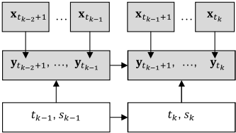
Fig.1 shows the graphical representation of our proposed model. It is a snapshot showing how segment k - 1 and k are related to each other. Our model consists of four major components.
The initial state model indicates the initial state probability at time 1
The transition model indicates the transition probability from state sk-1 to the next state sk:
Note that self-transition is not possible P (sk = i|sk-1 = i) = Aii = 0, because in that case there is only one segment instead of two. We note that some previous work [Kim and Smyth, 2006] specifies a fixed order of state transition (e.g., state 1 can only switch to state 2). In contrast, we allow arbitrary transitions between states.
The duration model specifies how long a state persists
In this work, we consider a poisson distribution. Other choices include geometric distribution and Gaussian distribution [Yu, 2010].
The observation model in general, assumes that the observation given a state follows a Gaussian distribution:
where fi(.) is mean and Vi is covariance. The main differences of previous approaches lies in the specification of function fi(.). For most HMM or HSMMmodels, fi(.) is assumed to be independent of time t (although fi(.) can depend on duration tk - tk-1 [Yu, 2010]). The previous segHMM improves this by defining fi(t) = ai + bit as a function of t [Kim and Smyth, 2006] or fi(t) = ai + cixt as a function of an input variable (covariate) xt [Chaubert-Pereira et al., 2010].
We consider a unified observation model defined as follows
Our model consists of three parts. The first part is a polynomial function with a order of R over time, the second part represents an autoregressive component with a order of Q and the last part depends on a L-dimensional input variable xt. h = [1 ... (t - tk-1)R y′t-1 ... y′t-Q xt,1, ..., xt,L]′ is a column vector with all known information at time t and θi = [ai,0 ... ai,R bi,1 ... bi,Q ci,1, ..., ci,L] contains all linear coefficients to be estimated. Note that θi is a matrix whose row dimension is equal to D, the dimension of yt. The autoregressive part is also referred to as vector autoregressive model (VAR) [L¨utkepohl, 1991]. We will not distinguish AR and VAR for the rest of this paper.
This unified observation model is the highlight of this paper as we fuse information from time, previous observations and input variables. Using input variables for condition monitoring and anomaly detection is a common practice [Song et al., 2007; Hayes and Capretz, 2014; Valko et al., 2011]. For example, for a gas turbine, gas flow, inlet guide vane (IGV) position (that controls the air flow) and inlet temperature can all be viewed as input sensors xt. They represent the inputs to the system and determine the values of other output sensors yt such as power, compressor temperatures and pressures, which are the main indicators of the performance and status of a gas turbine. The autoregressive part involving previous observations captures the dynamics of a machine, which provides extra information missed by using input variables alone. Finally, a failure often develops over time and exhibits a trending pattern. This is covered by the polynomial function over time in our model. If we exclude this polynomial component, to depict a trending pattern, we may have to use multiple states, one for each stage of the trend. Due to the additive nature of our model, we can easily add a new component if extra information is available or remove an existing component if it is not needed. This makes our model very flexible.
We have assumed a linear relationship between the parameters θi and constants h. The magnitude of the coefficient for a component indicates the importance of this component to the observation. This makes our model very interpretable. It is not difficult to extend fi(.) to a nonlinear function. For example, if we consider a Gaussian process [Rasmussen and Williams, 2006] with Gaussian kernel functions, all linear coefficients can be converted into the length scale parameters in the Gaussian kernel. However, in that case, the factorized form of (4) doesn't hold any more, therefore, the training complexity will be higher.
3.3 Training
During training, we are usually given N sequences. The n-th sequence consists of an output variable sequence Yn = y(n) 1:Tn and an input variable sequence Xn = x(n) 1:Tn . The task of training is to learn the parameters including initial state probability πi, transition probability Aij, duration parameter λi, observation model coefficients θi and covariance Vi, where i, j = 1, 2, ..., M. Let Ψ = {π, A, λ, θ, V} denote all parameters. We employ the Expectation-Maximization algorithm [Dempster et al., 1977] to learn Ψ by maximizing the log likelihood of all sequences logP(Y1:N, |X1:N,Ψ).
In the E-step, based on the current parameter estimation, we compute the following posterior distribution
The above procedure is often referred to as forward-backward algorithm [Rabiner, 1989; Yu, 2010]. All probabilities involved in (6) and (7) are defined in (1-4). It is important to view k as any segment (instead of the k-th segment) and k - 1 as its previous segment, because all parameters are not dependent on the the actual segment number (but only on its associated state sk). By integrating out the actual number of segments, we also reduce the complexity of the algorithm.
Once α(t(n) k , s(n) k ) and β(t(n) k , s(n) k ) are in place, it is straightforward to compute
Based on (8), we will compute posterior distributions that are directly used in the M-step.
(9) is used to estimate the parameters for the duration model (λ in (3)) and observation model (θ and V in (4)). (10) is used to estimate the parameters for the initial state model (π in (1)) and transition model (A in (2)). All parameters are estimated in analytical forms.
Pruning. We start the EM iterations with M = 10 states (obtained by randomly sampling training sequences). During EM iterations, we will prune a state if it is not supported by the data. Specifically, if a state i has a very low accumulative posterior probability ∑Nn=1 ∑Tn t=1 P (z(n) t = i|Yn) < 0.1, we will prune this state so the M can be reduced gradually. We found that using Poisson distribution for the duration model helps pruning (or merging of states). We initialize λi to being the average sequence length. This gives a broad prior for the duration such that the state whose observation model fits better will become more dominant. In contrast, using geometric distribution in the duration model doesn't have this property, because geometric distribution peaks at short duration and thus encourages shorter state (segment). For similar reasons, HMM doesn't have this nice property, either.
Numerical stability. The above algorithm as it often suffers numerical stability problems. The reason is that the EM iterations often involve multiplication of several exponential terms. If two such terms become extremely small or large, we may have an underflow or overflow problem, respectively. To overcome this, we compute both α(.) and β(.) in the log domain. The multiplication of two exponential terms exp(u) and exp(v) is simply u + v in the log domain. For adding two exponential terms, we take the maximum of u and v, which for example is u, and the result will be u + log(1 + exp(v - u)). This can be easily extended to operations involving more than two exponential terms. Once log P (t(n) k-1 , s(n) k-1 , t(n) k , s(n) k |Yn) is obtained in this way, we convert it back into the P(t(n) k-1 , s(n) k-1 , t(n) k , s(n) k |Yn) to complete the remaining EM computations.
Complexity. The complexity of training is O(NT 2M 2 ), where N is number of sequences, T is the maximum length of all sequences and M is the number of states. This is more expensive than O(NTM 2 ), the cost of training a HMM.
3.4 Monitoring
Once our model is trained, the standard way to find the best partition of a sequence is by using the Viterbi algorithm [Rabiner, 1989; Yu, 2010]. The complexity is O(T 2M 2 ) and it can be done online without iteration. We note that for realtime application, the most recent time t may not be the end of a segment as we have assumed in training. This situation is often referred to being right censored [Yu, 2010], in which we have to consider all possible ending point ≥ t for the current segment. The duration model will play a larger role in this situation, because we only have observations up to t. This will demand more training data to assure an accurate duration model. For our applications, relying more on the observation model than the duration model is more reasonable and thus we still assume that the current segment ends at t.
4 Test results
Under the unsupervised setting, many existing condition monitoring algorithms that require labels for training cannot be used. Therefore, we focus on comparing unsupervised HMMbased methods that are widely used and achieve impressive performances. Many such methods can be represented by our proposed unifying model. They differ by which information do we use in the observation component in (5). Let "HSMM", "t", "AR", "C" denote hidden semi-Markov model, using time component, using autoregressive component and using contextual component, respectively. Thus, in a t-AR-HSMMmodel, only time and autoregressive parts are used, i.e., ci,l in (5) is preset to zero. In a HSMM model, only ai,0 in (5) is used. We can similarly define other possible combinations. Note that t-HSMM is equivalent to segHMM. Our model can also be easily converted into hidden Markov models (HMM) by removing the duration model (thus no time component) and allowing self transition. For example, C-HMM means that only contextual part is used in the observation model.
Note that if a method, either HMM-based or HSMM-based, does not use input variables, we will append input variables xt to the end of yt. By doing this, different models are using the same data, but in a different way, either conditionally or jointly. All above models are implemented in matlab. For all tests conducted, we set the order of the polynomial function R = 1 and order of the autoregressive component Q = 1. The initial number of states is set to M = 10.
We conduct several tests to evaluate the performance of the proposed algorithm. These include two gas turbine data sets (from Siemens Energy), a truck data set (from Siemens Mobility) and the honeybee data set [Oh et al., 2008]. For test cases where we have ground truth label for every time stamp z∗ t , we can evaluate the performance of an algorithm quantitatively, as similarly done by other unsupervised techniques [Fox et al., 2009]. First, we convert the best partition obtained after the Viterbi algorithm into a label sequence zt. However, the label may not match that of z∗ t even if they correspond to the same segment. Therefore, for each ground truth label i, we find the corresponding label j produced by an algorithm that has the most overlap with i and map j to i. We repeat this for all ground truth labels. Note that this remapping doesn't change the segmentation result but only re-order its states. Finally, we define the classification rate Pc as Pc = ∑Tt=1 δ(zt-z∗ t ) T , where δ(zt - z∗ t ) = 1 if zt = z∗ t and zero otherwise. Unmatched labels either from ground truth or results all lead to classification errors.
4.1 Gas turbine performance data
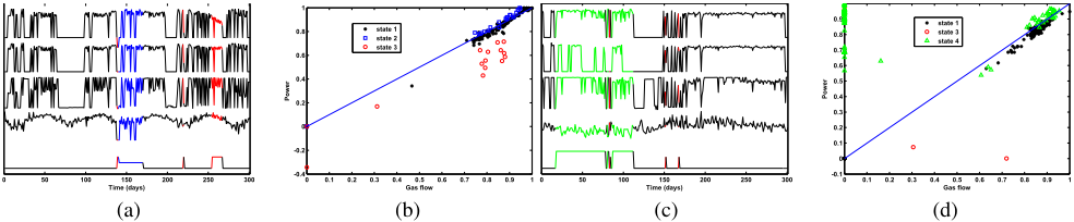
We consider six sequences from power generation. Each sequence represents a different gas turbine with about 10 months of operation data. The data resolution is one day. We focus on the power sensor as the output sensor yt (D = 1), because it is the most important performance indicator for a gas turbine. L = 3 input sensors including gas flow, IGV position and inlet temperature (Fig.2) are used.
Since we intend to learn behaviors of different machines jointly, data normalization is needed. One standard approach is to normalize each sensor to zero mean and unit variance. We instead normalize data by dividing each sensor over its corresponding maximum value. By doing this, we maintain the physical meaning of zero, which indicates a machine shutdown and this is true for all machines. If we use the standard normalization method, zero is likely to be converted to a negative value for shutdown period and can be different for different machines.
For this data set, we don't have ground truth labels. Our goal is to apply our t-AR-C-HSMM to blindly partition all six sequences, and find states indicating outliers and performance differences, shared through all units. After the EM algorithm converges, only M = 4 states remain while the other 6 are pruned by our algorithm automatically. Table 1 shows all estimated observation coefficients. Gas flow appears to have the most impact on power because its corresponding coefficient (ci,1 in the fifth column) is the highest for the first two states. Autoregressive coefficient (bi,1 in the fourth column) is the lowest, implying that power is quite independent from its previous value. This can be attributed to the low resolution we use: after one day, little dynamics is left.
| State i | ai,0 | ai,1 | bi,1 | ci,1 | ci,2 | ci,3 |
|---|---|---|---|---|---|---|
| 1 | 0.002 | 0.000 | 0.005 | 0.954 | 0.015 | -0.007 |
| 2 | -0.008 | 0.000 | 0.012 | 1.040 | 0.055 | -0.050 |
| 3 | 0.114 | -0.029 | -0.051 | 0.180 | 0.734 | 0.010 |
| 4 | 0.535 | -0.000 | 0.000 | -0.000 | 0.492 | -0.226 |
Figs.2(a) and 2(c) show sensor signals and our partition results for the first and fourth gas turbines, respectively. To make more sense out of the partition result, we show Figs.2(b) and 2(d) as well, where power is plotted against gas flow and different states are marked by different colors and symbols. This is a nice view to indicate the performance of a gas turbine. Typically, a higher power is desired given the same gas flow. A diagonal line is drawn to better visualize the performance difference. State 1 (black stars) appears to represent the most dominant mode (also see Fig.2(a)) of this gas turbine when the performance is slightly lower than the diagonal line. This is confirmed by its corresponding c1,1 = 0.954 (c1,1 = 1 representing the diagonal line) in Table 1. State 2 (blue squares) represents a higher efficiency with most data points above the diagonal line because of its c2,1 = 1.040.
State 3 clearly indicates an under-performing case. Power is much less correlated with gas flow and most data points are well below the diagonal line (red circles in Fig.2(b)). In addition, the first order polynomial coefficient a3,1 = -0.029 captures the downward trending of power around day 260 in the first plot of Fig.2(a). State 3 also covers some outlier time stamps when power is negative. This is unrealistic and could be due to sensor reading error.
State 4 is not shown in the first gas turbine, but has a significant presence in the fourth gas turbine (green curves or triangles in Figs.2(c) and 2(d)). A key characteristic of state 4
| Gas turbine | state 1 | state 2 | state 3 | state 4 |
|---|---|---|---|---|
| 1 | 0.847 | 0.100 | 0.053 | 0.000 |
| 2 | 0.963 | 0.027 | 0.010 | 0.000 |
| 3 | 0.037 | 0.957 | 0.006 | 0.000 |
| 4 | 0.694 | 0.000 | 0.010 | 0.296 |
| 5 | 0.199 | 0.000 | 0.000 | 0.801 |
| 6 | 0.944 | 0.000 | 0.056 | 0.000 |
is that we have power even when gas flow is zero (e.g., day 60 in Fig.2(c)). This again is likely due to sensor reading error. However, even when gas flow reading is normal (e.g., day 40 in Fig.2(c)), that data point is still classified as state 3. This can be attributed to the duration model that has a tendency to merge small segments into a big one if the resulting model error is tolerable.
Table 2 shows the percentage of four states in each of the six gas turbines. Based on the above analysis, we can conclude that the third gas turbine is the most efficient, because it has the most presence (0.957) of the most efficient state 2. The second gas turbine is mostly operating in the slightly less efficient state 1. Both the first and sixth gas turbine have about 0.05 of their time running in the very inefficient state 3. Therefore, a maintenance inspection should be suggested. The data from the fifth gas turbine appear to have many sensor reading errors because 0.801 of its time is in the unrealistic state 4. So a data cleaning is recommended.
4.2 Gas turbine failure data
In this section, we use gas turbine data containing a common failure due to cracks in the blade path component. This is usually reflected by a drop of the blade path temperatures. Typically, multiple (in our case eight) temperature sensors are installed in different locations of the blade path. The sensor closest to the crack will show the most obvious symptom and thus guide engineers to inspect that particular location. In this data set, there is one sequence with a resolution of 45 minutes. The beginning part of the sequence is normal and the failure shows in the last part. Therefore, we have ground truth with two states, one for normality and one for the failure.
We use D = 8 output sensors, all blade path temperature sensors as noted above and L = 3 input sensors including power, inlet temperature and the average of all output sensors. The last input variable is a calculated value, which is widely used in power generation. The basic assumption is that even if one temperature has deviation, the average temperature should still be stable and can be used to represent the normal behavior.
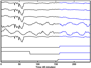
Fig.3 shows three output sensors and three input sensors. The third output sensor carries the failure symptom of a downward trending pattern at the end of the period. The ground truth labels, the partition results from a t-AR-HSMM and our model are also shown at the bottom. Classification rates for all models are shown in the third row of Table 3. Our model achieves the highest 0.980. We detect the failure slightly earlier than the ground truth annotated by the human expert (Fig.3), which may be more preferable. The t-AR-HSMM model creates an extra state at the begin of the sequence, which leads to a poor Pc = 0.680. This can be attributed to the following. Without using contextual component, the first part of the sequence (especially around day 60 in Fig.3) does look different from the rest. However, in the context of input sensors, the output sensors still follow the same state. This shows the benefit of using contextual information.
4.3 Truck data
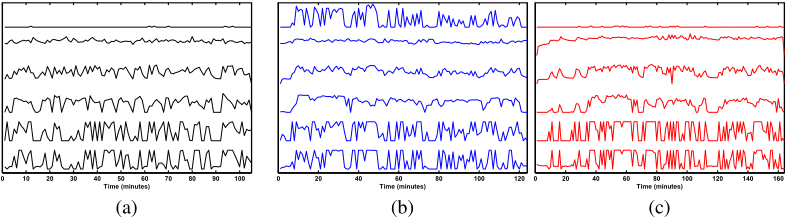
We use operation data from a truck. We consider two types of failures. The first type is caused by the failure of the exhaust filter, which results in a hike in exhaust air pressure. The second type is due to blocking of the grill, which leads to an increase of engine intake manifold temperature. Therefore, we use D = 2 input sensors including the exhaust air pressure and engine intake manifold temperature to identify these two failures. L = 7 other sensors including charge air cooler temperature, road speed, throttle, engine load, cooling temperature, ambient air temperature and altitude are used as input sensors.
There are N = 3 sequences used in this test, representing normality (ground truth state 1), exhaust filter failure (ground truth state 2), grill failure (ground truth state 3), respectively. Therefore, there is only one segment in each sequence. Each sequence has a resolution of one minute. Fig.4 shows all three sequences with two output sensors and the first four input sensors. The exhaust filter failure appears to be apparent: when it occurs, the exhaust air pressure (first plot in Fig.4(b)) is much higher than that in normal condition (first plot in Figs.4(a) and 4(c)). The grill blocking failure seems to be Time more subtle, because only a slight increase in engine intake manifold temperature is observable (second plot in Fig.4(c) compared to those in Figs.4(a) and 4(b)).
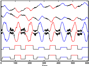
Figure 5: Honeybee data and results. The first four plots shows the honeybee's x, y coordinates and sine, cosine of its head angle. The last two plots show the ground truth partition, the partition found by our AR-HSMM model, respectively.
Our model and most other HSMM-based models are able to get perfect Pc = 1.000 for all three sequences (last three rows in Table 3). However, we note that t-HSMM gets Pc = 0.000 for the first sequence. A detailed check turns out that this model mis-classifies all data points in the first sequence to state 3. This suggests that using more evidence such as contextual information can increase modeling accuracy.
4.4 Honeybee data
This dataset has N = 6 sequences, each with D = 4 signals indicating the honeybee's x, y coordinates and sine, cosine of its head angle. Fig.5 shows all four signals of a sample sequence. There are three states to be identified: waggle, left turn and right turn, denoted by black, blue and red, respectively. This data set is not frommachine condition monitoring field, but is well studied by many time series segmentation algorithms.
Since there is no trending pattern within a state and no concept of contextual variables, we use AR-HSMM as our model. There are two settings to conduct the test. The first setting is unsupervised as we have been doing so far: an algorithm is trained using all six sequences without using any ground truth labels. The results are then evaluated against the ground truth. The second setting is supervised with a leaveone-out strategy: five sequences with the ground truth labels are used for training and the remaining sequence is for testing. Following [Fox et al., 2009], we fix the partitions for all five training sequences and learn our model. Then we apply the learned model with fixed parameter Ω to find the partition of the test sequence.
Table 4 shows the classification rate for all algorithms. In the supervised setting, SVM [Hoai et al., 2011] performs the best, possibly due to the nonlinear nature of a honeybee's trajectories. In the unsupervised setting, our results (last column) are better than those of [Fox et al., 2009; Hoai and Torre, 2012] but worse than that of [Zhou et al., 2013]. However, we note that both [Zhou et al., 2013] and [Oh et al., 2008] use domain knowledge specific to this problem in their model, which helps to improve their results.
| Models | HMM | AR-HMM | C-HMM | AR-C-HMM | HSMM | t-HSMM | AR-HSMM | C-HSMM | t-AR-HSMM | t-C-HSMM | AR-C-HSMM | t-AR-C-HSMM |
|---|---|---|---|---|---|---|---|---|---|---|---|---|
| Gas | 0.557 | 0.533 | 0.631 | 0.612 | 0.910 | 0.750 | 0.939 | 0.926 | 0.680 | 0.828 | 0.885 | 0.980 |
| Truck 1 | 0.847 | 0.943 | 1.000 | 0.838 | 1.000 | 0.000 | 1.000 | 1.000 | 1.000 | 1.000 | 1.000 | 1.000 |
| Truck 2 | 0.758 | 0.847 | 0.718 | 0.758 | 1.000 | 1.000 | 0.919 | 1.000 | 0.919 | 1.000 | 1.000 | 1.000 |
| Truck 3 | 0.634 | 0.927 | 0.945 | 0.512 | 1.000 | 1.000 | 1.000 | 1.000 | 1.000 | 1.000 | 1.000 | 1.000 |
| Test | [Oh] | [Hoai'11] | s-[Fox] | s-ours | [Fox] | [Hoai'12] | [Zhou] | Ours |
|---|---|---|---|---|---|---|---|---|
| 1 | 0.759 | 0.859 | 0.659 | 0.784 | 0.465 | 0.510 | 0.845 | 0.635 |
| 2 | 0.924 | 0.926 | 0.885 | 0.844 | 0.441 | 0.666 | 0.925 | 0.638 |
| 3 | 0.831 | 0.813 | 0.792 | 0.846 | 0.456 | 0.483 | 0.600 | 0.620 |
| 4 | 0.934 | 0.923 | 0.869 | 0.918 | 0.832 | 0.916 | 0.922 | 0.930 |
| 5 | 0.904 | 0.906 | 0.923 | 0.905 | 0.932 | 0.912 | 0.878 | 0.920 |
| 6 | 0.910 | 0.931 | 0.891 | 0.893 | 0.887 | 0.888 | 0.928 | 0.900 |
| Ave | 0.877 | 0.893 | 0.837 | 0.865 | 0.669 | 0.729 | 0.850 | 0.774 |
5 Summary
This paper tackles the machine condition monitoring problem under the unsupervised and multi-class setting, which is often neglected but becomes increasingly important in the era of big data. We present a new time series segmentation approach based on segmental hidden Markov model. We model the sensor observation as a unified function of three components including time, previous observations and contextual variables, which is proven to be suitable for machine condition monitoring. One big challenge of unsupervised approaches is how to interpret the results. Based on the intuitive meaning associated with the parameters, we show how the differences between states can indicate different operating modes and efficiencies of a machine. A variety of tests are conducted to show the effectiveness of the proposed model. Due to the additive nature of our observation model, we can easily introduce a new component if extra information is available or remove an existing component if it is not needed. This makes our model very flexible to be easily extended to other applications.
In this work, all coefficients in the observation model are free parameters. Overfitting doesn't appear to be a concern so far for two reasons. First, the parameters for each state are shared across segments and sequences (like a multi-task setting). Second, we keep the time and AR components rather simple by setting R = Q = 1. However, in some other applications, overfitting can occur with increasing model complexity or decreasing training set size. Parameter reduction techniques similar to LASSO [Jiang et al., 2012] and principal component analysis [Chang et al., 2014] have been introduced recently in several VAR-based approaches. One possible future direction of our model is to introduce regularization for variable selection as similarly done in [Jiang et al., 2012]. Our optimization objective will then consist of the log likelihood for the standard EM algorithm and this new regularization term. Another future direction is to extend our linear model to a nonlinear model such as Gaussian process [Rasmussen and Williams, 2006], as noted earlier. Gaussian process has a built-in mechanism for relevance determination.
Finally, although our training via the EM algorithm is much faster than MCMC-based algorithms and nonlinear segmentation algorithms, our algorithm still has a complexity proportional to T 2 , the square of a sequence length. This may become prohibitive for long sequences. One possible improvement is a multi-resolution coarse-to-fine approach that breaks an original sequence into many sub-sequences with multiple levels.
@inproceedings{ijcai2015p563,
  title     = {Unsupervised Machine Condition Monitoring Using Segmental Hidden Markov Models},
  author    = {Yuan, Chao},
  booktitle = {Proceedings of the Twenty-Fourth International Joint Conference on
               Artificial Intelligence, {IJCAI-15}},
  publisher = {International Joint Conferences on Artificial Intelligence},
  editor    = {Qiang Yang and Michael Wooldridge},
  pages     = {4009--4015},
  year      = {2015},
  month     = {7},
  note      = {Special Track on Machine Learning},
  url       = {https://ijcai.org/proceedings/2015/563},
}
TY - CPAPER TI - Unsupervised Machine Condition Monitoring Using Segmental Hidden Markov Models AU - Yuan, Chao T2 - Proceedings of the Twenty-Fourth International Joint Conference on Artificial Intelligence, IJCAI-15 PB - International Joint Conferences on Artificial Intelligence PY - 2015 SP - 4009 EP - 4015 UR - https://ijcai.org/proceedings/2015/563 ER -Copied
Machine-readable versions of this paper, for tools and AI agents:





