Bayesian Active Learning for Posterior Estimation - IJCAI-15 Distinguished Paper

1 Introduction

Computing the posterior distribution of parameters given observations is a central problem in statistics. We use the posterior distribution to make inferences about likely parameter values and estimate functionals of interest. For simple parametric models we may obtain the posterior in analytic form. In more complex models where the posterior is analytically intractable, we have to resort to approximation techniques. In some cases, we only have access to a black box which computes the likelihood for a given value of the parameters.

Our goal is an efficient way to estimate posterior densities when calls to this black box are expensive. This work is motivated by applications in computational physics and cosmology. Several cosmological phenomena are characterized by the cosmological parameters (e.g. Hubble constant, dark energy fraction). Given observations, we wish to make inferences about the parameters. Physicists have developed simulation-based probability models of the Universe which can be used to compute the likelihood of cosmological parameters for a given observation. Figure 1 shows different scenarios to estimate / compute the likelihood. Many problems in scientific computing have a similar flavour. Expensive simulators in molecular mechanics, computational biology and neuroscience are used to model many scientific processes.

Our contribution is to propose a query efficient method for estimating posterior densities when the likelihood function is expensive to evaluate. We adopt a Bayesian active regression approach on the log likelihood using the samples it has already computed. We refer to this approach as Bayesian Active Posterior Estimation (BAPE). We propose two myopic query strategies on the uncertainty regression model for sample selection. Our implementation uses Gaussian processes (GP) [Rasmussen and Williams, 2006] and we demonstrate the efficacy of the methods on multiple synthetic and real experiments.

2 RelatedWork

Practitioners have conventionally used sampling schemes [MacKay, 2003] to approximate the posterior distributions. Rejection sampling and various MCMC methods are common choices. The advantage of MCMC approaches is their theoretical guarantees with large sample sets [Robert and Casella, 2005] and thus they are a good choice when likelihood evaluations are cheap. However, none of them is intended to be query efficient when evaluations are expensive. Some methods spend most of their computation evaluating point likelihoods and then discard the likelihood values after doing an acceptance test. This gives insight into the potential gains possible by retaining those likelihoods for use in regression. Despite such deficiencies, MCMC remains one of the most popular techniques for posterior estimation in experimental science [Foreman-Mackey et al., 2013; Parkinson et al., 2006; Landau and Binder, 2005; Liu, 2001].

Approximate Bayesian computation (ABC) [Marin et al., 2012; Marjoram et al., 2003] is a method of last resort for estimating posteriors when a likelihood can not be computed. Unfortunately, it still requires the same generation of simulated data, which is expensive in our setup, and it does not address efficient selection of parameter values to be tested at all. Nested Sampling [Skilling, 2006] is a technique commonly used is Astrostatistics. Kernel Bayes' Rule [Fukumizu et al., 2014] is a non-parametric method of computing a posterior based on the embedding of probabilities in an RKHS. All these methods require sampling from a distribution and do not address the question of which samples to choose if generating them is expensive. The work in Bryan et al. [2006]

actively learns level sets of an expensive function and derives confidence sets from the results. Gotovos et al. [2013] also actively learn level sets via a classification approach. Our work is more general since we estimate the entire posterior.

Our methods draw inspiration from Gaussian Process based active learning methods such as Bayesian optimisation (BO) [Mockus and Mockus, 1991], Bayesian quadrature (BQ) [Osborne et al., 2012], active GP Regression (AGPR) [Seo et al., 2000] and several others [Srinivas et al., 2010; Gunter et al., 2014; Ma et al., 2014; Krause et al., 2008; Kandasamy et al., 2015]. These methods have a common modus operandi to determing the experiment θt at time step t: Construct a utility function ut based on the posterior GP conditioned on the queries so far. Then maximize ut to determine θt. ut(θ) captures the value of performing an experiment at point θ. Existing theoretical results [Golovin and Krause, 2011] justify such myopic strategies for homogeneous and stateless utility functions. Maximizing the typically multimodal ut is itself a hard problem. However, it is generally assumed that querying the function is more costly than this maximization [Brochu et al., 2010; Srinivas et al., 2010]. The key difference in such methods is essentially in the specification of ut to determine the next experiment. In our work, we adopt this strategy. We present two utility functions for active posterior estimation.

3 Bayesian Posterior Estimation

Problem Setting: We formally define our posterior distribution estimation problem in a Bayesian framework. We have a bounded continuous parameter space Θ for the unknown parameters (e.g. cosmological constants). Let Xobs denote our observations (e.g. signals from telescopes). For each θ ∈ Θ we have the ability to query an oracle for the value of the likelihood L(θ) = P(Xobs|θ), but these queries are expensive. Assuming a prior Pθ(θ) on Θ, we have the posterior Pθ|Xobs .

We wish to obtain an estimate ̂ Pθ|Xobs of Pθ|Xobs while minimizing our queries to the oracle.

Some smoothness assumptions on the problem are warranted to make the problem tractable. In the Bayesian framework it is standard to assume that the function of interest is a sample from a Gaussian Process. In what follows we shall model the log joint probability of the cosmological parameters and the observations via a GP 1 . This is keeping in line with Adams et al. [2008] who use a similar prior for GP density sampling and similar smoothness assumptions in Srinivas et al. [2010]. Assume that we have already queried the likelihood oracle at t - 1 points, and for each query point θi the oracle provided us with Li ≈ P(Xobs|θi) answers. Let At-1 = {θi, Li}t-1 i=1 denote the set of these input output pairs. We build our GP on Bt-1 = {θi, log(LiPθ(θi))}t-1 i=1 input output pairs. If g is a sample from this GP, then f = expg/ ∫ expg denotes a sample from the induced uncertainty model Fθ|Xobs for the posterior Pθ|Xobs . Finally, given any estimate ̂ P At (Xobs, θ) of the log joint probability, the estimate of the posterior distribution is,̂

At time t, we wish to select the point θt for the next experiment to evaluate the likelihood. We adopt a myopic strategy here by picking the point that maximizes a utility function. Our utility function needs to capture a measure of divergence D(·‖·) between the densities. To construct this utility function, note that ideally we would like to select θt to satisfy

where ̂ P At-1∪{(θ+,L(θ+))} is our estimate of the posterior using At-1 ∪ {(θ+,L(θ+))}. Obviously, this objective is not accessible in practice, since we know neither Pθ|Xobs nor L(θ+). As surrogates to this ideal objective in Equation (3), in the following subsections we propose two utility functions for determining the next point: Negative Expected Divergence (NED) and Exponentiated Variance (EV). The first, NED adopts a Bayesian decision theoretic approach akin to Settles [2010]. Here, we choose the point in Θ that yields the minimum expected divergence for the next estimate over the uncertainty model. Unfortunately, in our setting, the NED utility is computationally demanding. Therefore, we propose a cheaper alternative EV. In our experiments we found that both strategies performed equally well - so EV is computationally attractive. That said, some cosmological simulations are very expensive (taking several hours to a day) so NED is justified in such situations. We present our framework for BAPE using an appropriate utility function ut in Algorithm 1.

1 We work on the log joint probability since the log smoothes out a function and is more conducive for GP modeling. We also avoid issues such as non-negativity of ̂ P A m(θ|Xobs). Osborne et al. [2012] also use a similar log-transform before applying a GP.

Algorithm 1 Bayesian Active Posterior Estimation

Given: Input space Θ, GP prior µ0, k0.

For t = 1, 2, . . . do

1. θt = argmaxθt∈Θ ut(θ)
2. Lt ←Query oracle at θt.
3. Obtain posterior conditioned on (θi, LiPθ(θi))ti=1

3.1 Negative Expected Divergence (NED)

Equation 3 says that we should choose the point that results in the highest reduction in divergence if we knew the likelihood and the true posterior at that point. In NED, we choose the point with the highest expected reduction in divergence. For this we first build uncertainty models for the value of the likelihood at θ+ (L(θ+)) and the posterior (Fθ|Xobs ). For the next evaluation we choose the point that minimizes the expected divergence between these models and the next estimate. Precisely,

Here p+ is sampled from LA(θ+),the uncertainty of the likelihood at θ+. The density h is sampled from F A∪{(θ+,p+)} θ|Xobs , the uncertainty model of the posterior obtained by adding (θ+, p+). ̂ P A∪{(θ+,p+)} m+1 denotes the estimate of the posterior obtained by re-training the GP with (θ+, p+) as the (m+1)th point along with the m points already available. The first expectation above captures our uncertainty over L(θ+) while the second captures our remaining uncertainty over Pθ|Xobs after observing L(θ+). Equation (4) says that you should minimize the expected divergence by looking one step ahead.

The expectations in the NED utility above are computationally intractable. They can only be approximated empirically by drawing samples and require numerical integration. For these reasons we propose an alternate utility function below. In our experiments we found that both EV and NED performed equally well.

3.2 Exponentiated Variance (EV)

A common active learning heuristic is to choose the point that you are most uncertain about for the next experiment.

As before we use a GP on the log joint probability. At any given point in this GP we have an associated posterior variance of the GP. However, this variance corresponds to the uncertainty of the log joint probability whereas our objective is in learning the joint probability - which is a multiplicative factor away from the posterior. Therefore, unlike in usual GP active learning methods Seo et al. [2000], the variance of interest here is in the exponentiated GP. The posterior mean and variance at θ+ of our log-joint GP are given by,

where k(A,A) ∈ Rm×m is the kernel matrix of A, k(A, θ+) ∈ Rm is the kernel vector from θ+ to A and j = (log LiPθ(θi))mi=1 ∈ Rm. By observing that an exponentiated Gaussian is a log Normal distribution, the EV utility function is given by

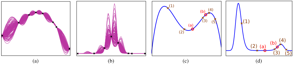
We choose the point maximizing the above variance. The exp(2µ(θ+)) will squash high variances in the low likelihood regions and amplify low variances in the high likelihood regions (Fig 2(a), 2(b)).

Its important to distinguish our objective in this work from similar active learning literature in the GP framework. In BO, the objective is to find the maximum of a function. This means that once the active learner realises that it has found the mode of a function it has less incentive to explore around as it would not improve the current maximum values. For instance, consider the log joint probability in Figure 2(c) and the joint probability in Figure 2(d). We have shown the points where we have already queried at as brown crosses and the red circles (a) and (b) show possible candidates for the next query. In BO, the active learner would not be interested in (b) as, by virtue of points (3), (4), (5) it knows that (b) is not likely to be higher than (4). On the other hand, in BAPE

we are keen on (b) as knowing it with precision will significantly affect our estimate of the posterior (Fig 2(d)). In particular to know the posterior well we will need to query at the neighborhood of modes and the heavy tails of a distribution. A BO utility is not interested in such queries. On the other extreme, in AGPR the objective is to learn the function uniformly well. This means in the same figures, AGPR will query point (a). However, given sufficient smoothness, the joint probability will be very low there due to exponentiation. Therefore, the BAPE active learner will not be interested in (a). As figures 2(a) and 2(b) indicate, while we model the log joint probability as a GP we are more interested in the uncertainty model of the posterior/ joint probability. Finally, as a special case for BQ, Osborne et al. [2012] consider evaluating the model evidence-i.e. the integral under the conditional. Their utility function uses approximations tailored to estimating the integral well. Note that our goal of estimating the posterior well is more difficult than estimating an integral under the conditional as the former implies the latter but not vice versa.

4 Other Algorithms for Comparison

We list some potential alternatives for posterior estimation and describe them here.

1. MCMC - Density Estimation (MCMC-DE): We implement MCMC with a Metropolis Hastings (MH) chain and use kernel density estimation (KDE) on the accepted points to estimate the posterior. When comparing MCMC against NED/EV we consider the total number of queries and not just those accepted. There are several variants of the MH proposal scheme and several tuning parameters. Comparing to all of them is nontrivial. We use MH in its basic form using a fixed Gaussian proposal distribution. Practitioners usually adjust the proposal based on the acceptance rate. Here, we chose the proposal manually by trying different values and picking the one that performed best within the queries used. Note that this comparison is advantageous to MCMC. In one experiment we test with Emcee [Foreman-Mackey et al., 2013], a popular package for Affine Invariant MCMC which automatically fine tunes the proposal bandwidth based on acceptance rate [Foreman-Mackey et al., 2013].

2. MCMC - Regression (MCMC-R): Here, as in MCMCDE we use a MH Chain to generate the samples. However, this time we regress on the queries (not samples) to estimate the posterior. We include this procedure since MCMC can be viewed as a heuristic to explore the parameter space in high likelihood regions. We show that a principled query strategy outperforms this heuristic.

3. Approximate Bayesian Computing (ABC): There are several variants of ABC [Marjoram et al., 2003; Peters et al., 2012]. We compare with a basic form given in Marin et al. [2012]. At each iteration, we randomly sample θ from the prior and then sample an observation Xsim from the likelihood. If d(Xsim,Xobs) < ϵ we add θ to our collection. Here d(·, ·) is some metric on a sufficient statistic of the observation and ϵ > 0 is a prespecified threshold. We perform a KDE on the collected samples to estimate the posterior. The performance of ABC depends on ϵ: As for MCMC-DE we choose ϵ by experimenting with different values and choosing the value which gives the best performance within the queries used. We compare with total number of parameter values proposed and not just those retained.

4. Uniform Random Samples (RAND): Here, we evaluate the likelihood at points chosen uniformly on Θ and then regress on these points.

5 Experiments

We first look at a series of low and high dimensional synthetic and real astrophysical experiments. NED is only tested on low dimensional problems since empirical approximation and numerical integration is computationally expensive in high dimensions. Further, since the inner expectation in Equation (4) is expensive we approximate it using a one sample estimate. We use a squared exponential kernel in all our experiments. The bandwidth for the kernel was set to be 5n-1/d where n is the total number of queries and d is the dimension. This was following several kernel methods (such as kernel

regression) which use a bandwidth on the order O(n -c1 c2+d ) [Gy¨orfi et al., 2002]. Other kernel hyperparameters was set via cross validation every 20 iterations. In our experiments, EV slightly outperforms NED probably since the EV utility can be evaluated exactly while NED can only approximated. We omit most technical details of the experiments due to space constraints.

Low Dimensional Synthetic Experiments:

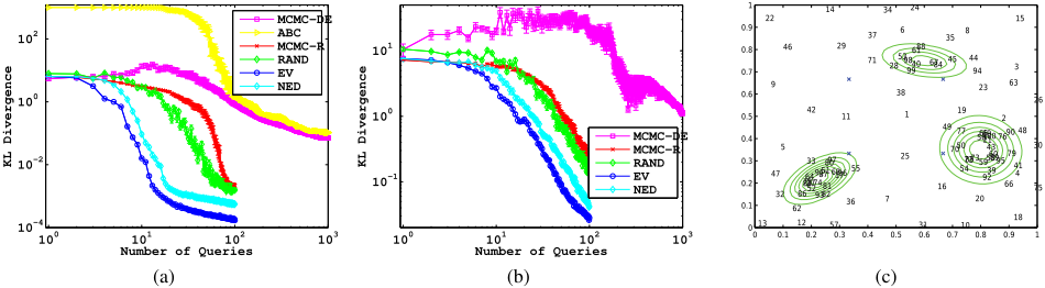
To illustrate our methods we have two simple yet instructive experiments. In the first, the parameters space is Θ = (0, 1) equipped with a Beta(1.2, 1) prior. We draw θ from the prior, and then draw 500 samples from a Bernoulli(θ2 + (1 - θ)2 ) distribution: i.e. Xobs ∈ {0, 1}500 . The ambiguity on the true value of θ creates a bimodal posterior. Figure 3(a) compares NED/EV against the other methods as a function of the number of queries. The second is a 2D problem with Θ = (0, 1)2 . Here we artificially created a 3-modal log-joint posterior shown by green contours in Figure 3(c). Figure 3(b) compares all methods. As we artificially constructed the log likelihood ABC does not apply here. Figure 3(c) shows the points chosen by the NED query strategy in order. It shows that we have learned the high log joint probability regions well at the expense of being uncertain at low log joint probability areas. However, this does not affect the posterior significantly as they are very small after exponentiation. Our proposed methods outperform existing methods and other heuristics by orders of magnitude on these simple experiments.

Higher Dimensional Synthetic Datasets:

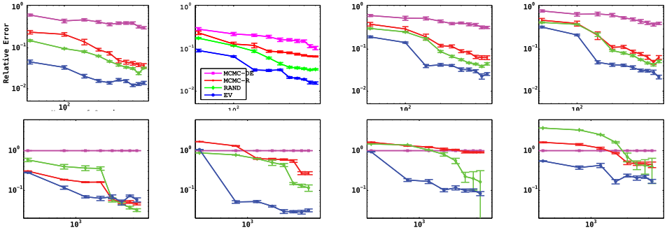
We test in d = 5 and 15 dimensions. We construct an artificial log likelihood so that the resulting posterior is mixture of 2 Gaussians centred at 0 and 1. We evaluate performance by the ability to estimate certain linear functionals. The exact value of these functionals can be evaluated analytically since we know the true posterior.

We use a uniform prior. Our log-likelihood is, ℓ(θ) = log(0.5N(θ; 0, 0.5√dI) + 0.5N(θ; 1, 0.5√dI)). Our functionals are T1 = E ∑di=1 Xi, T2 = E ∑di=1 X2 i , T3 = E ∑d-1 i=1 X2 i Xi+1 and T4 = E ∑d-2 i=1 XiXi+1Xi+2. For MCMC-DE, we draw samples Z1, Z2, . . . from the true likelihood. To estimate Ti = Eφi(X) we use the empirical estimator ̂ Ti = 1/N ∑k φi(Zk). For EV , MCMC-R and RAND we first use the queried points to obtain an estimate of the loglikelihood by regressing on the likelihood values as explained before. Then we run an MCMC chain on this estimate to collect samples and use the empirical estimator for the functionals. Note that evaluating the estimate, unlike the likelihood, is cheap. ABC does not apply in this experiment. The results are shown in Figure 4. They demonstrate the superiority of our query strategy over the alternatives.

Type Ia Supernovae:

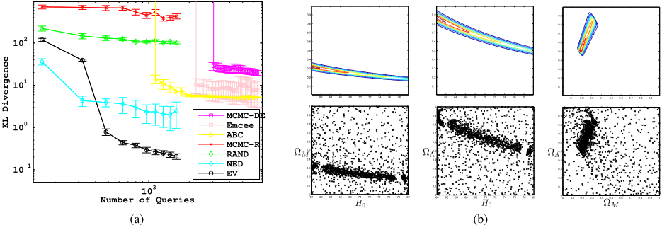
We use supernovae data for inference on 3 cosmological parameters: Hubble Constant (H0 ∈ (60, 80), Dark Matter Fraction ΩM ∈ (0, 1) and Dark Energy Fraction ΩΛ ∈ (0, 1). The likelihood for the experiment is given by the RobertsonWalker metric which models the distance to a supernova given the parameters and the observed red-shift. The dataset is taken from Davis et al [2007]. The parameter space is taken to be Θ = (0, 1)3 (For H0 we map it to (60, 80) using an appropriate linear transform). We test NED/EV against MCMC-DE, ABC, MCMC-R, RAND and Emcee. For ABC, sampling from the likelihood is as expensive as computing the likelihood. Figure 5(a) compares all methods. Figure 5(b) shows the points queried by EV and the marginals of the true posterior. The KL for RAND decreases slowly since it accumulates points at the high likelihood region very slowly. MCMC-R performs poorly since it has only explored part of the high likelihood region. For NED/EV after an initial exploration phase after which the error shoots down.

Luminous Red Galaxies:

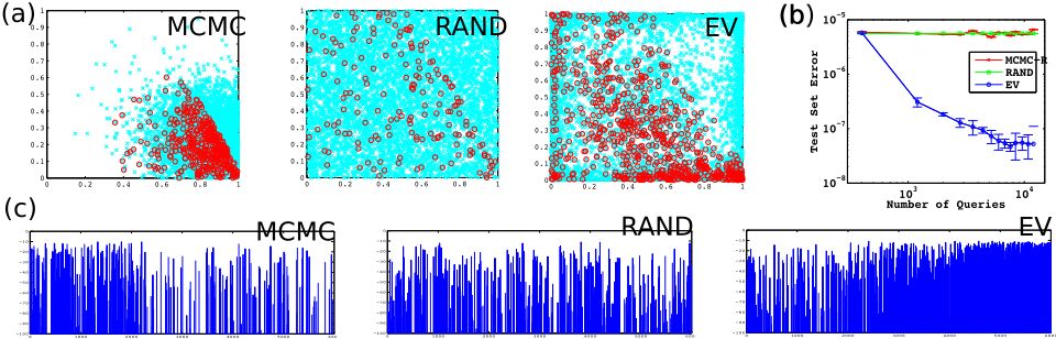
Here we used data on Luminous Red Galaxies (LRGs) for inference on 8 cosmological parameters. We use software and data from Tegmark et al [2006]. Our parameter space is taken to be (0, 1)8 by appropriately linear transforming the range of the variables. Each query takes about 4-5 seconds. In EV determining the next point takes about 0.5-1 seconds with ≈ 2000 points and about 10-15 seconds with ≈ 10000 points. In this regime, EV is wall clock time competitive with other methods. ABC does not apply in this experiment.

Fig. 6a shows points queried by MCMC, RAND and EV projected on the first 2 dimensions. MCMC has several high likelihood points but its queries are focused on a small region of the space. RAND does not have many points at high likelihood regions. EV has explored the space fairly well and at the same time has several queries at high likelihood regions. Fig 6c shows the evaluated log likelihood at each query. It shows that as predicted EV first explores the space (high likelihood queries are sparse) and then exploits the high likelihood regions. Since ground truth is difficult to obtain for this experiment, we perform the following simple test. We queried 250, 000 points uniformly at random from the parameter space to form a test set. We then run EV, MCMC-R and RAND for up to 12, 000 queries to collect points and estimate the posterior. Performance is evaluated by the mean squared reconstruction error of the exponentiated log joint probabilities (joint probabilities). Figure 6b shows the results. The error for RAND and MCMC-R stay the same throughout since the problem is difficult and they did not have sufficient number of high likelihood points throughout the space.

6 Conclusions

We proposed a framework for query efficient posterior estimation for expensive blackbox likelihood evaluations. Our methods use GPs and are based on popular ideas in Bayesian active learning. We demonstrate that our methods outperform natural alternatives in practice.

Note that in Machine Learning it is uncommon to treat posterior estimation in a regression setting. This is probably since the estimate will depend on the intricacies of the regression algorithm. So if likelihood evaluations are inexpensive, MCMC seems a natural choice due to its theoretical guarantees in the large sample regime. However, our work demonstrates that when likelihood evaluations are expensive, such as in scientific simulations, treating posterior estimation in an active regression framework enables us to be significantly query efficient.

Acknowledgement: This research was partly funded by DOE grant DESC0011114.