Lightweight Temporal Description Logics with Rigid Roles and Restricted TBoxes

1 Introduction

Classical description logics (DLs), such as those underlying the W3C standard OWL, are a successful family of knowledge representation languages. Temporal description logics (TDLs) extend classical DLs, providing built-in means to represent and reason about temporal aspects of knowledge. The importance of TDLs stems from the need of relevant applications to capture temporal and dynamic aspects of knowledge, e.g., in medical and life science ontologies, which are very large but still demand efficient reasoning, such as SNOMED CT and FMA [Bodenreider and Zhang, 2006], and the gene ontology (GO) [The Gene Ontology Consortium, 2000]. A natural task is to model dynamic knowledge about patient histories against static medical knowledge (e.g., about diseases): e.g., the temporal concept C := E✸∃ requiresTransfusion.⊤ describes a patient who may need a blood transfusion in the future, and the axiom Anemic ⊑ C says that this applies to anemic people. In contrast, Anemia ⊑ Disorder represents static knowledge.

A notable approach to designing TDLs is to combine DLs with temporal logics commonly used in software/hardware verification such as LTL, CTL(∗) , and to provide a twodimensional product-like semantics [Schild, 1993; Gabbay et al., 2003; Lutz et al., 2008]. The combination allows various design choices, e.g., we can restrict the scope of temporal operators to certain types of entities (such as concepts, roles, axioms), or declare some DL concepts or roles as rigid, meaning that their interpretation will not change over time. The need for rigid roles in TDL applications, e.g., in biomedical ontologies to accurately capture life-time relations, has been identified [Baader et al., 2008]. For example, the role hasBloodType should be rigid since a human's blood type does not change during their lifetime.

Unfortunately, TDLs based on the Boolean-complete DL ALC with rigid roles cannot be effectively used since they become undecidable as soon as temporal operators are applied to concepts and a general TBox is allowed [Gabbay et al., 2003; Guti´errez-Basulto et al., 2014]. This is the case even if we severely restrict the temporal operators available and use the sub-Boolean DL EL, whose standard reasoning problems are tractable, instead of ALC [Artale et al., 2007a; Guti´errezBasulto et al., 2014]. In the light of these results, several efforts have been devoted to the design of decidable TDLs with rigid roles [Artale et al., 2007b; 2014]; e.g., decidability can be attained by using a different lightweight DL component based on DL-Lite. Both the EL and DL-Lite families underlie prominent profiles of the OWL standard.

Interestingly, no research has been yet devoted to TDLs based on EL in the presence of restricted TBoxes, such as classical TBoxes, which consist solely of definitions of the form A ≡ C with A atomic and unique, or acyclic TBoxes, which additionally forbid syntactic cycles in definitions. This is surprising since in the presence of general TBoxes TDLs based on EL tend to be as complex as the ALC variant [Artale et al., 2007b; Guti´errez-Basulto et al., 2012; 2014].

These considerations lead us to investigating TDLs with rigid roles based on EL and the (branching-time) CTL allowing for temporal concepts and empty or acyclic TBoxes. We strongly believe that TDLs designed in this way are wellsuited as temporal extensions of biomedical ontologies. After all, large parts of SNOMED CT and GO indeed are acyclic EL-TBoxes.

Our main contributions are algorithms for standard reasoning problems and (mostly tight) complexity bounds. We begin by showing that the combination of CTL and ALC with empty and acyclic TBoxes is decidable. Our nonelementary upper bound is optimal even when the set of temporal operators is restricted to E✸ ("possibly eventually") or E© ("possibly next"). We then replace ALC with EL and maintain the restriction to E✸, E© and empty TBoxes. We particularly show that the resulting TDLs are decidable in PTIME with one of the two operators, and CONP-complete with both. To this aim, we employ canonical models, together with expansion vectors [Haase and Lutz, 2008] in the case with both E✸, E©. Next, we lift the PTIME upper bound to the case of acyclic TBoxes, employing a completion algorithm in the style of those for EL and extensions, [Baader et al., 2005]. Finally, we show that the combination of E✸ with A✷ ("always globally") and acyclic TBoxes leads to a PSPACE-complete TDL, again employing a completion algorithm. An overview of existing and new results is given in Table 1, where CTLYX denotes the combination of the DL X with the fragment of CTL restricted to the temporal operators Y . In particular, all the new results hold even if rigid concepts are also included.

Table 1: Overview of previous and new complexity results. ≥ hardness, ≤ membership, = completeness

The relatively low complexity that we obtain for EL-based TDLs over restricted TBoxes are in sharp contrast with the undecidability and nonelementary lower bounds known for the same logics over general TBoxes [Guti´errez-Basulto et al., 2014]. With the restriction to acyclic TBoxes, we will thus identify the first computationally well-behaved TDLs with rigid roles based on EL and classical temporal logics.

Due to limited space, additional technical notions and proofs are in a report: http://tinyurl.com/ijcai15tdl

2 Preliminaries

We introduce CTLALC , a TDL based on the classical DL ALC. Let NC and NR be countably infinite sets of concept names and role names, respectively. We assume that NC and NR are partitioned into two countably infinite sets: N rig C and N loc C of rigid concept names and local concept names, respectively; and, N rig R and N loc R of rigid role names and local role names, respectively. CTLALC-concepts C are defined by the grammar

where A ranges over NC, r over NR. We use standard DL abbreviations [Baader et al., 2003] and temporal abbreviations E✸C, A✷C, A✸C and A(C U D) [Clarke et al., 1999].

The semantics of classical DLs, such as ALC, is given in terms of interpretations of the form I = (∆, ·I ), where ∆ is a non-empty set called the domain and ·I is an interpretation function that maps each A ∈ NC to a subset AI ⊆ ∆ and each r ∈ NR to a binary relation rI ⊆ ∆×∆. The semantics of CTLALC is given in terms of temporal interpretations based on infinite trees [Guti´errez-Basulto et al., 2014]: A temporal interpretation based on an infinite tree T = (W,E) is a structure I = (T, (Iw)w∈W) such that, for each w ∈ W, Iw is a DL interpretation with domain ∆; and, rIw = rIw′ and AIw = AIw′ for all r ∈ N rig R , A ∈ N rig C and w,w′ ∈ W. We usually write AI,w instead of AIw . The stipulation that all worlds share the same domain is called the constant domain assumption (CDA). For Boolean-complete TDLs, CDA is the most general: increasing, decreasing and varying domains can all be reduced to it [Gabbay et al., 2003, Prop. 3.32]. For the sub-Boolean logics studied here, CDA is not w.l.o.g. Indeed, we identify a logic in which reasoning with increasing domains cannot be reduced to the constant domain case.

We now define the semantics of CTLALC-concepts. A path in T = (W,E) starting at a node w is an infinite sequence π = w0w1w2 · · · with w0 = w and (wi,wi+1) ∈ E. We write π[i] for wi, and use Paths(w) to denote the set of all paths starting at the node w. The mapping ·I,w is extended from concept names to CTLALC-concepts as follows.

An acyclic CTLALC-TBox T is a finite set of concept definitions (CDs) A ≡ D with A ∈ NC and D a CTLALC concept, such that (1) no two CDs have the same left-hand side, and (2) there are no CDs A1 ≡ C1, . . . , Ak ≡ Ck in T such that Ai+1 occurs in Ci for 1 ≤ i ≤ k, where Ak+1 = A1.

A temporal interpretation I is a model of a concept C if C I,ε ̸= ∅; it is a model of an acyclic TBox T , written I |= T , if AI,w = C I,w for all A ≡ C in T and w ∈ W; it is a model of a concept inclusion C ⊑ D, written I |= C ⊑ D, if C I,w ⊆ DI,w for all w ∈ W.

The two main reasoning tasks we consider are concept satisfiability and subsumption. A concept C is satisfiable relative to an acyclic TBox T if there is a common model of C and T . A concept D subsumes a concept C relative to an acyclic TBox T , written T |= C ⊑ D, if I |= C ⊑ D for all models I of T . If T is empty, we write |= C ⊑ D.

3 First Observations

We start by observing that the combination of CTL and ALC with rigid roles relative to empty and acyclic TBoxes is decidable and inherently nonelementary. In a nutshell, we show the upper bounds using a variant of the quasimodel technique [Gabbay et al., 2003, Thm. 13.6]; the lower bound follows from the fact that satisfiability for the product modal logics S4×K and K×K is inherently nonelementary [G¨oller et al., 2015]. Indeed, the fragment of CTLALC allowing E✸ (E©) as the only temporal operator is a notational variant of S4×K (K×K) [Guti´errez-Basulto et al., 2014].

Theorem 1 Concept satisfiability relative to acyclic and empty TBoxes for CTLALC with rigid roles is decidable and inherently nonelementary.

With Theorem 1 and the third column of Table 1 in mind, we particularly set as our goal the identification of elementary (ideally tractable) TDLs. To this aim, we study combinations of (fragments of) CTL with the lightweight DL EL. CTLEL is the fragment of CTLALC that disallows the constructor ¬ (and thus the abbreviations C ⊔D, ∀r.C, A✷, . . . ). The standard reasoning problem for CTLEL, as for EL, is concept subsumption since each concept and TBox are trivially satisfiable. In what follows we consider various fragments of CTLEL obtained by restricting the available temporal operators. We denote the fragments by putting the allowed operators as a superscript. In this context, we view each of the operators E✸, A✷ as primitive instead of as an abbreviation.

In order to keep the presentation of our main results accessible, in Sections 5-6, we concentrate on the case where only rigid role names and local concept names are present. Later on, in Section 7, we explain how to deal with the general case.

4 CTLE◦,E✸ EL relative to the Empty TBox

We begin by investigating the complexity of subsumption relative to the empty TBox for a TDL whose subsumption relative to general TBoxes is undecidable: CTLE◦,E✸ EL .

Theorem 2 Concept subsumption relative to the empty TBox is CONP-complete for CTLE◦,E✸ EL with rigid roles and in PTIME for CTLE◦ EL and CTLE✸ EL with rigid roles.

CONP-hardness is obtained by embedding EL plus transitive closure into CTLE◦,E✸ EL ; the jump in complexity comes from the ability to express disjunctions, e.g., |= E✸C ⊑ C ⊔ E©E✸C. We next explain CONP-membership; the PTIME results are a byproduct and improved later.

We proceed in two steps: first we provide a characterization of |= C ⊑ D where C is an CTLE◦ EL -concept and D an CTLE◦,E✸ EL -concept. Next we generalize this characterization to CTLE◦,E✸ EL -concepts C.

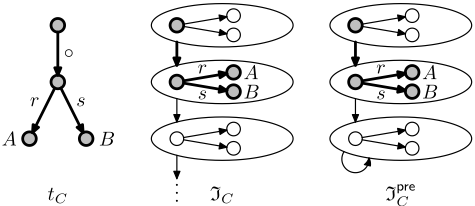
Given a CTLE◦ EL -concept C, the description tree tC = (VC, LC, EC) for C is a labeled graph corresponding to C's syntax tree; we denote its root by xC. For example, if C = E©(∃r.A ⊓ ∃s.B), then tC is given in Figure 1, left.

For plain EL, we have |= C⊑D if and only if there is a homomorphism from tD to tC, which can be tested in polynomial time [Baader et al., 1999]. This criterion cannot directly be transferred to CTLE◦ EL because tC does not explicitly represent all pairs of worlds and domain elements whose existence is implied by tC, e.g., for |= E©∃r.A ⊑ ∃r.E©A with r rigid, there is no homomorphism from tD to tC. We overcome this problem by transforming tC into a canonical model IC of C, i.e., (1) its distinguished root is an instance of C and (2) IC homomorphically embeds into every model of C. The construction of IC from tC is straightforward: for every node with an incoming ©-edge (r-edge, r being a role) create a fresh world (domain element); for the root xC create both a world and domain element. The temporal relation and the interpretation of r and concept names is read off EC and LC. To transform (W,R) into an infinite tree, we add an infinite path of fresh worlds to every world without R-successor. The canonical model for the above concept C is shown in Fig. 1, center; the infinite path of worlds is dashed.

From (1), (2), and the preservation properties of homomorphisms, we obtain the desired characterization of subsumption.

Lemma 3 For all CTLE◦ EL -concepts C and all CTLE◦,E✸ EL - concepts D, we have |= C ⊑ D if and only if xC ∈DIC,xC .

Now xC ∈ DIC,xC can be verified by model-checking D in world xC and element xC of I pre C , which is the polynomialsized modification of I where the lastly added infinite path of worlds is replaced by a single loop, see Figure 1, right. Since IC is the unraveling of I pre C into the temporal dimension, both interpretations satisfy the same concepts in their roots. Theorem 2 for CTLE◦ EL therefore follows. The CTLE✸ EL part can be obtained by representing every E✸ in C by a ©-edge in tC and modifying the notion of a homomorphism.

For CTLE◦,E✸ EL , we use expansion vectors introduced by Haase and Lutz [2008], applied to the temporal dimension. Let C be a CTLE◦,E✸ EL -concept with n occurrences of E✸. An expansion vector for C is an n-tuple U = (u1, . . . , un) of natural numbers ui ∈ N (including 0). Intuitively, U fixes a specific number of temporal steps taken for each E✸ in C when constructing tC and IC. More precisely, we use C[U] to denote the CTLE◦ EL -concept obtained from C by replacing the i-th occurrence of E✸ with (E©)ui , that is, a sequence of ui E©-operators. For example, if C = E✸∃r.E✸(A ⊓E©B) and U = (2, 0), then C[U] = E©E©∃r.(A ⊓ E©B).

Let UmC be the set of all expansion vectors (u1, . . . , un) with 0 ⩽ ui ⩽ m, for all i = 1, . . . , n. We denote with td(D) the nesting depth of temporal operators in D. We use expansion vectors with entries bounded by td(D) to reduce ̸|= C ⊑ D for CTLE◦,E✸ EL to the case where C is fromCTLE◦ EL .

Lemma 4 For all CTLE◦,E✸ EL -concepts C,D, we have

Together with Lemma 3, this yields the desired polynomialtime guess-and-check procedure for deciding |= C ⊑ D.

5 CTLE◦ EL and CTLE✸ EL relative to Acyclic TBoxes

The results of Theorem 2 transfer to acyclic TBoxes with an exponential blowup due to unfolding [Nebel, 1990], that is:

Corollary 5 Concept subsumption relative to acyclic CTLE◦,E✸ EL -TBoxes with rigid roles is in CONEXPTIME.

For the subfragments CTLE◦ EL and CTLE✸ EL , we can even show polynomial complexity as in the empty TBox case.

Theorem 6 Concept subsumption relative to acyclic CTLE◦ EL - and CTLE✸ EL -TBoxes with rigid roles is in PTIME.

We first concentrate on the E✸ case and explain below how to deal with the E© one. We focus w.l.o.g. on subsumption between concept names and assume that the input TBox is in normal form (NF), i.e., each axiom is of the shape A ≡ A1 ⊓ A2, A ≡ E✸A1, or A ≡ ∃r.A1, where Ai ∈ NC ∪ {⊤} and r ∈ NR. As usual, a subsumption-equivalent TBox in NF can be computed in polynomial time [Baader, 2003]. We use CN and ROL to denote the sets of concept names and roles occurring in T .

To prove a PTIME upper bound, we devise a completion algorithm in the style of those known for EL and (twodimensional) extensions, cf. [Baader et al., 2005; Guti´errezBasulto et al., 2011], which build an abstract representation of the 'minimal' model of the input TBox T (in the sense of Horn logic). The main difficulty is that different occurrences of the same concept name in the TBox cannot all be treated uniformly (as it is the case for, say, EL), due to the two-dimensional semantics. Instead, we have to carefully choose witnesses for E✸A and ∃r.A, respectively. Our algorithm constructs a graph G = (W,E,Q,R) based on a set W, a binary relation E, a mapping Q that associates with each A ∈ CN and each w ∈ W a subset Q(A, w) ⊆ CN, and a mapping R that associates with each rigid role r ∈ ROL a relation R(r) ⊆ CN × W × CN × W. For brevity, we write (A,w) r→ (B,w′ ) instead of (A,w,B,w′ ) ∈ R(r) and denote with E∗ the reflexive, transitive closure of E.

The algorithm for deciding subsumption initializes G by setting R(r) = ∅ for all r ∈ ROL and for all A ∈ CN:

Intuitively, the unraveling of (W,E) is the temporal tree underlying the canonical model and the mappings Q and R contain condensed information on how to interpret concepts and roles, respectively. More specifically, the data stored in Q(A, ·) describes the temporal evolution of an instance of A. For example, Q(A,AA) collects all concept names B such that T |= A ⊑ B; likewise, Q(A,E✸A) captures everything

• F1 If B∈Q(A,AA′ ) &B ≡ E✸B′ ∈ T , add (AA′,AB′ ) to E
• F2 If B ∈ Q(A,w) and B ≡ ∃r.B′ ∈ T , set (A,w) r→ (B′ ,B′B′ )
• F3 If B∈Q(A,w) &B≡A1⊓A2 ∈T , add A1,A2 to Q(A,w)
• C1 If (BB,w) ∈ E and (A,w′ ) r→ (B,BB), add (w′,w) to E
• C2 If (A,w) r→ (B,BB), then
• (A,w′ ) r→ (B,E✸B) for all w′ ̸= w with (w′,w) ∈ E∗
• (A,w′ ) r→ (B,w′ ) for all w′ with (w′ ,w) /∈ E∗
• B1 If B ∈ Q(A, w), (w′ , w) ∈ E∗ , and A′ ≡ E✸B ∈ T , add A′ to Q(A,w′ )
• B2 If A ∈ Q(B,w), (A′ ,w′ ) r→ (B,w), and A′′ ≡ ∃r.A ∈ T add A′′ to Q(A′ ,w′ )
• B3 If A1,A2 ∈ Q(B,w) &A ≡ A1 ⊓A2 ∈ T add A to Q(B, w)

Figure 2: Completion rules

that follows from E✸A. Finally, Q(A,AB) contains concept names that are implied by B given that B appears in the temporal evolution of an instance of A, i.e., B′ ∈ Q(A, AB) implies T |= A⊓E✸B ⊑ E✸(B ⊓B′ ).

After initialization, the algorithm extends G by applying the completion rules depicted in Figure 2 in three phases. In the first phase - also called FORWARD-phase, since definitions A ≡ C ∈ T are read as A ⊑ C - rules F1-F3 are exhaustively applied in order to generate a fusion-like representation by adding witness-worlds and witness-existentials as demanded. Most notably, rule F2 introduces a pointer to the structure representing the temporal evolution of an instance of B′ .

Subsequently, G is extended to conform with the constant domain assumption and reflect rigidity of roles by exhaustively applying rules C1 and C2. For example, one can read C2 as 'if two points are connected via r in some world, then they should be connected in all worlds.' Note that Q(B, E✸B) is used as a representative for the entire "past" of B in part a).

In the final phase, BACKWARD-completion rules B1-B3 are exhaustively applied in order to respect the 'backwards'- direction of definitions, i.e., definitions A ≡ C ∈ T are read as A ⊒ C. This separation into a FORWARD and BACKWARD phase is sanctioned by acyclicity of the TBox. In fact, one run through each phase is enough; note that no new tuples are added to E or R in the BACKWARD-phase.

The following lemma shows correctness of our algorithm.

Lemma 7 Let T be an acyclic CTLE✸ EL -TBox in normal form. Then for all A,B ∈ CN, we have T |= A ⊑ B iff, after exhaustive rule application, B ∈ Q(A, AA).

For proving "⇐", we show that (a certain unraveling of) G "embeds" into every model of A and T . For this purpose, we need to adapt the notion of a homomorphism to temporal interpretations and rigid roles. For the reverse direction, we construct from G a model I of T such that d ∈ AI,w \ BI,w for some d,w. It is not hard to see that the algorithm runs in polynomial time: The size of the data structures W, E, and R is clearly polynomial and the mapping Q(·, ·) is extended in every rule application, so the algorithm stops after polynomially many steps.

Finally, we sketch two modifications of the algorithm such that it works for E© instead of E✸. First, we have to use a non-transitive version of B1. Second, and a bit more subtly, we have to replace E✸A ∈ W with E©kA, 1 ≤ k ≤ |T | to capture what is implied by E©kA; more precisely, B′ ∈ Q(A,E©kA) implies T |= E©kA ⊑ B′ , where E©k denotes E© · · · E© k times.

We next show that there is a jump in the complexity if increasing domains are considered instead of constant ones. Intuitively, this can be explained by the fact that increasing domains allow rigid roles to mimic the behaviour of the A✷- operator. In the next section, we show that the addition of A✷ to {E✸} indeed leads to PSPACE hardness.

Theorem 8 Concept subsumption relative to acyclic CTLE◦ EL - and CTLE✸ EL -TBoxes with rigid roles and increasing domains is PSPACE-hard.

6 CTLE✸,A✷ EL relative to Acyclic TBoxes

We now add A✷ and observe that this leads to an increase in complexity to polynomial space over acyclic TBoxes.

Theorem 9 Concept subsumption relative to acyclic CTLE✸,A✷ EL -TBoxes with rigid roles is PSPACE-complete.

The lower bound is obtained via a reduction from QBF validity. For the upper bound, we again consider w.l.o.g. subsumption between concept names and assume that the acyclic TBox is in normal form, i.e., axioms are of the shape A ≡ A1 ⊓A2, A ≡ E✸A1, A ≡ A✷A1, or A ≡ ∃r.A1, where Ai ∈ NC ∪ {⊤} and r ∈ NR. We also restrict ourselves again to only rigid roles. CN and ROL are used as before.

In contrast to the previous section, we cannot maintain the entire minimal model in memory since the added operator A✷ can be used to enforce models of exponential size. Instead, we will compute all concepts implied by the input concept A (the left-hand side of the subsumption to be checked) by iteratively visiting relevant parts of the minimal model. Our main tool for doing so are traces.

Definition 1 A trace is a tuple (σ,E,R) where σ is a sequence (d0,w0) · · · (dn,wn) such that for all 0 ≤ i < n one of the following is true:

• di = di+1 and (wi, wi+1) ∈ E;
• wi = wi+1 and (di, di+1) ∈ R(r) for some r ∈ ROL.

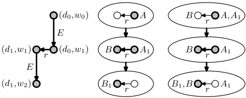
Intuitively, traces represent paths through temporal interpretations, which in each step follow either the temporal relation (first item of Definition 1) or a DL relation r (second item of Definition 1); so, in a pair (d,w), d can be thought of as a domain element and w as a world.

Our algorithm, whose basic structure is depicted in Algorithm 1, enumerates on input A and T , in a systematic tableaulike way, all traces that must appear in every model of A and T . It is important to note that in the context of Algorithm 1 a trace is used as the basis for inducing a richer structure that conforms with the constant domain assumption and captures rigidity; see Example 1 below. The algorithm also maintains an additional mapping Q that labels each point (d, w) of the

Algorithm 1: Subsumption in CTLE✸,A✷ EL

Input: Acyclic TBox T , concept names A, B Output: true if T |= A ⊑ B, false otherwise 1 σ := (d0,w0); Q(d0,w0) := {A,⊤}; 2 E := ∅; R(r) := ∅ for all r ∈ ROL; 3 expand(σ,E,R); 4 return true if B ∈ Q(d0,w0), false otherwise; 5 procedure expand (σ,E,R) : 6 complete (σ,E,R,Q); 7 if (σ,Q) is periodic at (i, j) then 8 add (wj-1, wi) to E; 9 truncate; 10 complete (σ, E, R, Q); 11 return; 12 (d,w) := last element of σ; 13 foreach A ∈ Q(d, w) with A ≡ ∃r.B ∈ T do 14 Q(d′ , w) = {B, ⊤} for a fresh d′ ; 15 add (d, d′ ) to R(r); 16 expand (σ · (d′ , w), E, R); 17 foreach A ∈ Q(d, w) with A ≡ E✸B ∈ T do 18 Q(d, w′ ) = {B, ⊤} for a fresh w′ ; 19 add (w, w′ ) to E; 20 expand (σ · (d, w′ ), E, R);

trace (and all the induced points) with a set Q(d,w) ⊆ CN. The set Q(d, w) captures all concept names that are satisfied in the minimal model at points represented by (d, w).

The basics of Algorithm 1 are the following. In Lines 1 and 2, it creates a trace consisting of a single point representing A and initializes the necessary data structures. In Line 3, the systematic expansion is set off. When that is finished, the algorithm just returns whether or not B (the right-hand of the subsumption) has been added during the expansion. As for the expand procedure:

• in Line 6 and 10, the algorithm updates the mapping Q;
• Line 7 contains some termination condition; and finally,
• the loops in Lines 13 and 17 enumerate all ∃r.B and E✸B that appear in the set Q(d, w) of the last element of the trace and expand the trace to witness these concepts.

This basic description of the algorithm leaves open several points: (i) the precise behavior of the subroutine complete, (ii) when a trace is periodic, and (iii) what happens inside the truncate command in Line 9. Let us start with describing the subroutine complete. It uses additional mappings Qcert(d) ⊆ CN and QA✷(d, w) ⊆ CN, which intuitively contain all the concept names that d satisfies certainly, i.e., in all worlds, and starting fromworld w, respectively. It proceeds in two steps:

1. Initialize undefined Q(d,w) and Qcert(d) with {⊤}, and undefined QA✷(d, w) with Qcert(d); and
2. apply rules R1-R12 in Figure 3 to Q(·), Qcert(·) and QA✷(·).

The number of rules is indeed scarily high; however, they can be divided into four digestible groups: R1 and R2 are used

• R1 If A ≡ A1 ⊓A2 ∈ T and A ∈ Q∗(·), add A1,A2 to Q∗(·)
• R2 If A ≡ A1 ⊓A2 ∈ T and A1,A2 ∈ Q∗(·), add A to Q∗(·)
• R3 If (d, d′ ) ∈ R(r), B ∈ Q(d′ , w), A ≡ ∃r.B ∈ T , add A to Q(d, w)
• R4 If B ∈ Q(d,w), (w′ ,w) ∈ E∗ , A ≡ E✸B ∈ T , add A to Q(d, w′ )
• R5 If B ∈ Q(d,w), (w,w′ ) ∈ E∗ , B ≡A✷A ∈ T , add B, A to Q(d, w′ )
• R6 If (d, d′ ) ∈ R(r), B ∈ Qcert(d′ ), A ≡ ∃r.B ∈ T , add A to Qcert(d)
• R7 If B ∈ Qcert(d), A ≡A✷B ∈ T , add A to Qcert(d)
• R8 If B ∈ Qcert(d), add B to Q(d, w) for all w
• R9 If B ∈ QA✷(d,w), A ≡A✷B ∈ T , add A to Q(d,w)
• R10 If A ∈ Q(d, w), A ≡ A✷B ∈ T , add A, B to QA✷(d, w)
• R11 If (d, d′ ) ∈ R(r), B ∈ QA✷(d′ , w), A ≡ ∃r.B ∈ T , add A to QA✷(d, w)
• R12 If A ∈ QA✷(d, w), A ≡ E✸B ∈ T , w′ added due to A ∈ Q(d, w) in Line 18, B′ ∈ Q(d, w′ ), A′ ≡ E✸B′ ∈ T , add A′ to QA✷(d,w)

Figure 3: Saturation rules, where in R1 and R2 the set Q∗(·) ranges over all Q(d, w), Qcert(d), and QA✷(d, w).

to ensure that all sets Q∗ are closed under conjunction; R3R5 are used to complete Q(·). Note that R1-R4 are already known from the algorithm of the previous section. Furthermore, R6-R8 are used to deal with Qcert(·); and R9-R12 to update QA✷(·). As an example of the interplay between the different mappings take R9: If B is certain for d starting in world w and A ≡ A✷B, then we also know that d satisfies A in w; and R11 for the interplay between temporal operators and rigid roles: indeed, for r rigid, |= ∃r.A✷B ⊑A✷∃r.B.

Example 1 Let T ={A≡E✸A1, A1 ≡∃r.B, B≡E✸A1} be the input TBox; and T |= A ⊑ A1 is to be checked. Figure 4 (left) shows the trace initiated at (d0,w0) with Q(d0, w0) = {⊤, A}, and further expanded in Lines 13 and 17. The trace, as mentioned above, induces a richer structure, reflecting rigid roles and the constant domain assumption; see Fig. 4 (center). This richer structure is then completed to properly enrich the types Q(d, w) of each element. In particular, during completion, further concept names are added to the corresponding types (Fig. 4, right). One can now easily see that T |= A ⊑ A1 indeed holds. Furthermore, note that T ̸|= A ⊑ A1, if r is local or increasing domains are assumed. This is the case since, in both cases, the r-connection is not necessarily present in the 'root world'.

For the termination condition in Line 7, we take the following definition of periodicity.

Definition 2 A trace (σ, E, R) together with a mapping Q is called periodic at (i, j) if σ = (d0,w0) · · · (dn,wn), i < j, di = dj = dn, and Q(di, wi) = Q(dj , wj ).

This means that during the evolution of element d = di = dj , we find two different worlds wi, wj such that d has the same type in wi and wj. We can stop expanding worlds appearing after wj since their behavior is already captured by the successors of wi. If a trace periodic at (i, j) is found, we add an edge (wj-1,wi) to E reflecting the periodic behavior, see Line 8. Then, in truncate, the trace is shortened to (d0,w0) · · · (dj-1,wj-1) and the relations E and R(r), r ∈ ROL, and the mappings Q,Qcert,QA✷ are restricted to those d and w that appear in the shortened trace.

Lemma 10 On every input T , A, B, Algorithm 1 terminates and returns true iff T |= A ⊑ B.

For termination, consider a trace with suffix (d, w1) · · · (d, wn) and let additionally A1, . . . ,An be the concept names such that E✸Ai lead to wi, see Line 17 of Algorithm 1. It is not difficult to show that if Ai = Aj for i < j, then Q(d,wi) ⊆ Q(d, wj) after application of complete. Since Q(d, w) ⊆ CN, there are no infinite (strictly) increasing sequences. Hence, the expansion in Lines 17ff. will not indefinitely be applied. Also, the expansion in Lines 13ff. stops due to acyclicity of the TBox. Together, this guarantees termination.

Correctness is shown similar to Lemma 7. For "⇒", we show that every trace together with the labeling so far computed in Q can be embedded into every model of A and T . For "⇐", we present a model of T witnessing T ̸|= A ⊑ B.

To finish the proof of Theorem 9, it remains to note that the termination argument indeed yields a polynomial bound on the length of the traces encountered during the run of Algorithm 1.

7 Local Roles and Rigid Concepts

One can easily extend the above algorithms so as to deal with local roles. In fact, e.g., in Section 5 only B4 in Figure 5 needs to be added to the BACKWARD-rules in Figure 3. Note that F2 is only applied to rigid roles and C2 is therefore not applied to local ones. Clearly, the algorithm in Section 6 can be extended with a similar rule.

Recall that rigid concepts are concepts whose interpretation does not change over time. In the first example from Section 1, the concept Disorder should be rigid because we consider medical knowledge as static. In contrast, PatientWithDisorder should be local because a disease history has a begin and end.

In the presence of general TBoxes, rigid concepts can be simulated by rigid roles: replace each rigid concept name A with ∃rA.⊤, where rA is a fresh rigid role. Unfortunately, this simulation does not work in the context of acyclic TBoxes since the result of replacing A with ∃rA.⊤ in a CD A ≡ D is not a CD anymore. Nevertheless, our algorithms can be extended, without increasing the complexity, to consider rigid B4 If A ∈ Q(B,w), A ≡ ∃r.A′ , B′ ∈ Q(A′ ,A′A′ ) and B′′ ≡ ∃r.B′ ∈ T , add B′′ to Q(B, w)

RC If B ∈ Q(A, w), B ∈ CNrig, add B to Q(A, w′ ), ∀w′ ∈ W

R13 If B ∈ Q(d,w) or B ∈ QA✷(d,w) &B ∈ CNrig, then add B to Qcert(d)

Figure 5: Rules for Local Roles and Rigid Concepts

concepts: e.g., the algorithm in Section 5 can be extended by adding RC above to the FORWARD and BACKWARD rules - CNrig denotes the set of rigid concepts occurring in the input TBox. Note that the intermediate phase remains the same, i.e., rules C1 and C2 are neither extended nor modified.

Rigid concepts can analogously be included in Section 6 by adding R13 to the rules in Figure 3. Recall that, intuitively, Qcert(d) contains the concepts that hold for d in any world.

Finally, note that in the empty TBox case rigid roles can indeed simulate rigid concepts, as described above.

8 Conclusions and FutureWork

In this paper we have initiated the investigation of TDLs based on EL allowing for rigid roles and restricted TBoxes. We indeed achieved our main goal: we identified of fragments of the combination of CTL and EL that have elementary, some even polynomial, complexity.

One important conclusion is that the use of acyclic TBoxes, instead of general ones, allows to design TDLs based on EL with dramatically better complexity than the ALC variant; e.g., for the fragment allowing only E© the complexity drops from nonelementary to PTIME. As an important byproduct, the studied fragments of CTLEL can be seen as positive fragments of product modal logics with elementary complexity, e.g., implication for the positive fragment of K×K is in PTIME.

As a next step, we plan to look at more expressive fragments of CTLEL or at classical (cyclic) TBoxes, e.g., consider nonconvex fragments, such as CTLE◦,E✸ EL , with (a)cyclic TBoxes. We plan to incorporate temporal roles, too. It is also worth exploring how restricting TBoxes can help tame other TDLs with bad computational behavior over general TBoxes, such as TDLs based on LTL or the µ-calculus. We believe that the LTL case is technically easier than ours since it does not have the extra ' 12 -dimension' introduced by branching.

Acknowledgements The first author was supported by the M8 PostDoc Initiative project TS-OBDA and the second one by the DFG project LU1417/1-1. We thank the anonymous reviewers for their detailed and constructive suggestions.