
Maximum Satisfiability Using Cores and Correction Sets
Proceedings of the Twenty-Fourth International Joint Conference on Artificial Intelligence. Main Track. Pages 246-251.
© 2015 International Joint Conferences on Artificial Intelligence
Abstract
Core-guided MAXSAT algorithms dominate other methods in solving industrial MAXSAT problems. In this work, we propose a new efficient algorithm that is guided by correction sets and cores. At every iteration, the algorithm obtains a correction set or a core, which is then used to rewrite the formula using incremental and succinct transformations. We theoretically show that correction sets and cores have complementary strengths and empirically demonstrate that their combination leads to an efficient MAXSAT solver that outperforms state-of-the-art WPMS solvers on the 2014 Evaluation on industrial instances.
- [Aavani et al., 2013] Amir Aavani, David G. Mitchell, and Eu- genia Ternovska. New encoding for translating pseudo- boolean constraints into sat. In Alan M. Frisch and Peter Gregory, editors, SARA. AAAI, 2013.
- [Ansótegui et al., 2013] Carlos Ansótegui, Maria Luisa Bonet, and Jordi Levy. SAT-based MaxSAT algorithms. Artificial Intelligence, 196:77-105, 2013.
- [Bacchus et al., 2014] Fahiem Bacchus, Jessica Davies, Maria Tsimpoukelli, and George Katsirelos. Relaxation Search: A Simple Way of Managing Optional Clauses. In Proceedings of the 28th Conference on Artificial intelligence (AAAI'14), pages 2717-2723, 2014.
- [Belov et al., 2012] Anton Belov, Ines Lynce, and Joao Marques-Silva. Towards efficient mus extraction. AI Com- mun., 25(2):97-116, 2012.
- [Belov et al., 2013] Anton Belov, Huan Chen, Alan Mishchenko, and Joao Marques Silva. Core minimiza- tion in SAT-based abstraction. In Design, Automation and Test in Europe (DATE), pages 1411-1416. ACM, March 2013.
- [Cimatti et al., 2010] Alessandro Cimatti, Anders Franzen, Al- berto Griggio, Roberto Sebastiani, and Cristian Stenico. Sat- isfiability modulo the theory of costs: Foundations and ap- plications. In Javier Esparza and Rupak Majumdar, editors, [Cooper et al., 2006]
- Martin C. Cooper, Sylvain Cussat-Blanc, Marie de Roquemaurel, and Pierre Regnier. Soft Arc Con- sistency Applied to Optimal Planning. In Frederic Ben- hamou, editor, Proceedings of the 12th International Con- ference on Principles and Practice of Constraint Program- ming (CP'06), volume 4204 of Lecture Notes in Computer Science, pages 680-684. Springer, 2006.
- [Een and Sorensson, 2003] Niklas Een and Niklas Sorensson. An extensible SAT-solver. In Enrico Giunchiglia and Ar- mando Tacchella, editors, Proceedings of the 6th Interna- tional Conference on Theory and Applications of Satisfiabil- ity Testing (SAT'03), volume 2919, pages 502-518. Springer, 2003.
- [Grac ¸a et al., 2012] Ana Grac ¸a, Inês Lynce, João Marques- Silva, and Arlindo L. Oliveira. Efficient and accurate haplo- type inference by combining parsimony and pedigree infor- mation. In Proceedings of the 4th International Conference on Algebraic and Numeric Biology, pages 38-56, Berlin, Heidelberg, 2012. Springer-Verlag.
- [Heras et al., 2011] Federico Heras, António Morgado, and João Marques-Silva. Core-Guided Binary Search Algorithms for Maximum Satisfiability. In AAAI, 2011.
- [Ignatiev et al., 2014] Alexey Ignatiev, António Morgado, Vasco M. Manquinho, Inês Lynce, and João Marques-Silva. Progression in maximum satisfiability. In Proceedings of the 21th European Conference on Artificial Intelli- gence(ECAI'14), pages 453-458, 2014.
- [Juma et al., 2012] Farah Juma, Eric I. Hsu, and Sheila A. McIlraith. Preference-based planning via maxsat. In Pro- ceedings of the Canadian Conference on Artificial Intelli- gence, pages 109-120, 2012.
- [Manquinho et al., 2009] Vasco M. Manquinho, Joao P. Mar- ques Silva, and Jordi Planes. Algorithms for weighted Boolean optimization. In Oliver Kullmann, editor, Proceed- ings of the 12th International Conference on Theory and Ap- plications of Satisfiability Testing (SAT'09), volume 5584, pages 495-508. Springer, 2009.
- [Marques-Silva and Planes, 2008] Joao Marques-Silva and Jordi Planes. Algorithms for maximum satisfiability using unsatisfiable cores. In DATE, pages 408-413. IEEE, 2008.
- [Martins et al., 2014] Ruben Martins, Saurabh Joshi, Vasco Manquinho, and Inês Lynce. Incremental Cardinality Con- straints for MaxSAT. In International Conference on Princi- ples and Practice of Constraint Programming. LNCS, 2014.
- [Morgado et al., 2012] Antonio Morgado, Federico Heras, and Joao Marques-Silva. Improvements to core-guided binary search for MaxSAT. In Alessandro Cimatti and Roberto Se- bastiani, editors, Proceedings of the 15th International Con- ference on Theory and Applications of Satisfiability Testing (SAT'12), volume 7317, pages 284-297. Springer, 2012.
- [Morgado et al., 2013] António Morgado, Federico Heras, Mark H. Liffiton, Jordi Planes, and Joao Marques-Silva. It- erative and core-guided MaxSAT solving: A survey and as- sessment. Constraints, 18(4):478-534, 2013.
- [Morgado et al., 2014] António Morgado, Carmine Dodaro, and Joao Marques-Silva. Core-guided maxsat with soft car- dinality constraints. In Principles and Practice of Constraint Programming -20th International Conference, CP 2014, Lyon, France, September 8-12, 2014. Proceedings, pages 564-573, 2014.
- [Narodytska and Bacchus, 2014] Nina Narodytska and Fahiem Bacchus. Maximum satisfiability using core-guided maxsat resolution. In Proceedings of the 28th Conference on Artifi- cial intelligence (AAAI'14), pages 2717-2723, 2014.
- [Parrain, 2010] Daniel LeBerre Anne Parrain. The sat4j library, release 2.2. JSAT, 7(2-3):59-6, 2010.
- [Rosa and Giunchiglia, 2013] Emanuele Di Rosa and Enrico Giunchiglia. Combining approaches for solving satisfia- bility problems with qualitative preferences. AI Commun., 26(4):395-408, 2013.
- [Strickland et al., 2005] Dawn M. Strickland, Earl Barnes, and Joel S. Sokol. Optimal protein structure alignment using maximum cliques. Oper. Res., 53(3):389-402, May 2005.
- [Vasquez and Hao, 2001] Michel Vasquez and Jin-Kao Hao. A "logic-constrained" knapsack formulation and a tabu algo- rithm for the daily photograph scheduling of an earth obser- vation satellite. Comp. Opt. and Appl., 20(2):137-157, 2001.
References were extracted automatically from the PDF and may contain errors.
Full text extracted automatically from the PDF; figures, tables and equations may differ. The PDF is the version of record.
Introduction
Maximum Satisfiability (MAXSAT) is an optimisation version of satisfiability (SAT) that contains both hard clauses and weighted soft clauses. A solution of MAXSAT is an assignment that satisfies all hard clauses and violates a minimum weight subset of soft clauses. Many industrial applications can be naturally encoded in MAXSAT. Successful application areas include bioinformatics [Strickland et al., 2005; Grac¸a et al., 2012], planning and scheduling [Cooper et al., 2006; Vasquez and Hao, 2001; Juma et al., 2012].
There exist a number of different approaches to solving MAXSAT. The most successful approach for industrial problems performs iterative solving using a SAT solver as an oracle on each iteration [Morgado et al., 2013; Ans´otegui et al., 2013]. Existing solvers differ in how they perform optimal cost estimation, e.g. linear or binary search, and the kind of information they use to estimate the cost, e.g. cores, the structure of cores, or satisfying assignments. While there are many algorithms that perform search on either upper bound or lower bound of the optimal cost [Ans´otegui et al., 2013; Morgado et al., 2013; Narodytska and Bacchus, 2014; Morgado et al., 2014], there are very few algorithms that efficiently perform combined search over two bounds, e.g. [Heras et al., 2011; Ignatiev et al., 2014]. The current state-of-the-art approach for combined search performs binary-like search over the range of possible cost values, which can be exponentially more efficient than linear search. However, one of the drawbacks of binary search-based algorithms is that they modify
Nina Narodytska
Carnegie Mellon University Pittsburgh, USA ninan@cs.cmu.edu
the formula using expensive PseudoBoolean (PB) constraints, while, for example, the lower bound-based linear search does not introduce PB constraints. PB constraints increase the size of the formula and, potentially, slow down the solver.
We present an efficient and robust algorithm that takes advantage of lower and upper bounds estimates. Our approach is in the spirit of linear search [Marques-Silva and Planes, 2008], as we create a sequence of SAT problems. A key strength of our algorithm is that it uses succinct formula transformations that do not use PB constraints and can be applied incrementally. Our algorithm is based on a fundamental duality between cores and correction sets. In each incremental step it arbitrates between cores and correction sets making low overhead progress towards optimality. Experimental results demonstrate the potential of this approach: our PRIMALDUALMAXSAT solver, shows robust performance and outperforms the best WPMS algorithms on industrial instances by a noticable margin.
Background
A satisfiability problem consists of a set of clauses φ = {C1, . . . ,Cm} over a set of Boolean variables X. A literal l is either a variable xi ∈ X or its negation xi. A clause C is a disjunction of literals (l1 ∨⋯∨ ln). A unit clause is a clause containing only one literal. We denote the set of variables in the formula φ by vars(φ). An assignment I of the variables vars(φ) is a mapping vars(φ) ↦ {0, 1}, extended to literals by I(x) = 1 - I(x), clauses I(C) = max{I(l) ∣ l ∈ C}, and sets of clauses φ, by I(φ) = min{I(C) ∣ C ∈ φ}. If I(φ) = 1, then I is a solution to the satisfiability problem φ.
A weighted clause is a pair (C,w), where C is a clause and w is the weight of C, w ∈ N ∪ {∞}, that gives the cost of violating C. Clauses with w = ∞ are called hard clauses; otherwise, the clause is a soft clause. A Weighted Partial MAXSAT (WPMS) Problem consists of a set of a set of weighted clauses, φ = {(C1,w1), . . . , (Cm,wm)}. A special case of WPM is Partial MAXSAT (PMS), where the problem weights are in the set {1,∞}. We denote the set of soft clauses in φ by softCls(φ) and the set of hard clauses by hardCls(φ). W.l.o.g., we can assume that soft clauses (C, w) in φ are unit clauses (b, w) as φ can be converted to this form by introducing reification variables: φ = [φ ∖ {(C,w)}] ∪ {(C ↔ b), (b,w)}. We also assume standard clausification, e.g., C↔b denotes {(b ∨ C)} ∪ ⋃l∈C{(l ∨ b)}.
An assignment I is feasible for φ iff I satisfies all hard clauses of φ. The cost of I is the sum of weights of clauses that it falsifies: cost(I,φ) = ∑(b,w)∈φ∧I(b)=0 w. I is an optimal assignment for φ iff it is a feasible assignment of minimal cost. We denote this minimal cost by cost(φ) = minI is feasible cost(I,φ). The maximal finite cost is maxcost (φ) = ∑(b,w)∈φ∧w<∞ w.
To simplify notation, we omit weights for hard clauses and we assume they are satisfiable. A ϕ ⊆ φ is a core of φ iff ϕ is unsatisfiable. A core ϕ is minimal iff ∀(b,w) ∈ ϕ, ϕ ∖ {(b, w)} is a satisfiable formula. A π ⊆ φ is a correction set iff φ∖π is satisfiable. A correction set π is minimal iff ∀(b, w) ∈ π φ ∖ (π ∖ {(b, w)}) is unsatisfiable.The cost of a correction set π is maxcost(π). A smallest minimal correction set π is a minimum correction set. We denote I(φ) the set of solutions of φ. A solution I corresponds to a correction set π iff I(bi) = 0 for (bi) ∈ π and I(bi) = 1 otherwise.
Related work
There are two main classes of SAT-based algorithms for solving MAXSAT [Morgado et al., 2013]. Algorithms in the first class perform linear search on the value of the cost. It can be partitioned into two subclasses. The first subclass of solvers perform so called UNSAT-SAT search (LBLINEAR), e.g. [Ans´otegui et al., 2013; Manquinho et al., 2009; Narodytska and Bacchus, 2014; Morgado et al., 2014]. They start with an unsatisfiable formula and gradually increase the lower bound on the optimal cost by performing a sequence of relaxations of the formula. The second subclass of solvers perform so called SAT-UNSAT search (UBLINEAR). They start with a satisfiable formula and perform a sequence of strengthenings on it [Parrain, 2010; Martins et al., 2014]. The second class combines upper and lower bound searches by performing binary or linear search on the cost value [Cimatti et al., 2010; Heras et al., 2011; Morgado et al., 2012; Marques-Silva and Planes, 2008; Ignatiev et al., 2014].
The work [Marques-Silva and Planes, 2008] is the most relevant to us as it performs lower and upper bound search. The main distinction of our approach is in how we transform the formula based on using a core or a correction set. In particular, we do not use PB constraints in our transformations.
PRIMALDUALMAXSAT algorithm
We first present our algorithm for unweighted partial MAXSAT, so that all soft clauses have weight one. The weighted case, solved using cloning, is discussed later.
The algorithm searches for cores and correction sets of the formula simultaneously by performing a sequence of SAT calls. At each step the algorithm detects either a core or a correction set. However, we do not know in advance which of two will be found and let our search procedure decide on this. The algorithm terminates in at most m steps, which is the same worst case guarantee as linear search algorithms. The algorithm uses two phases: a partition and a transformation phase. Algorithm 1 shows the pseudocode. Core minimization (line 23) is optional. It does not affect correctness. Let us detail the two phases.
Partition. The algorithm partitions all soft clauses into two sets ϕi and πi at the ith round. The first set of soft clauses must be satisfied along with the hard clauses and the second set of clauses can be violated at this round. We call ϕi a candidate core and πi a candidate correction set. Note that by splitting soft clauses, we guarantee that either ϕi is a valid core or πi a valid correction set. The main question here is how to perform partitioning of the clauses. Our idea is inspired by relaxation search [Rosa and Giunchiglia, 2013; Bacchus et al., 2014]. Relaxation search branches on variables from soft clauses positively. Using unit propagation, these decisions may force other variables to be falsified. After all variables from soft clauses are instantiated (Algorithm 1, lines 7-10), we have a candidate core ϕi = {b ∣ I(b) = 1} and a candidate correction set πi = {b ∣ I(b) = 0}. We call the SAT solver in the context of hardCls(φi ), and partial assignment I in line 13 to determine satisfiability of hardCls(φi ) ∣I . If hardCls(φi ) ∣I is UNSAT then it returns a subset of ϕi as a valid core; otherwise πi is a valid correction set.
The partition phase has several useful properties. First, if the solver is satisfiable using a candidate set π, then it is minimal (Proposition 2 in [Bacchus et al., 2014]). So there is no need to reduce it. Second, suppose I(b) = 0 is implied during the partition phase. Then {b} ∪ {b′ ∣ I(b′ ) = 1} is a core of φ. In this case, if checking whether π is a correction set is computationally expensive, we can apply the primal transformation to this core. Third, suppose I is a partial assignment such that ∣{b ∣ I(b) = 0}∣ > ub. Then I is not going to be extended to a minimal solution. In this case, we can block this assignment and resume the search. We omit these extensions in our pseudocode.
Transformation. The transformation phase takes as input a core or a correction set. If hardCls(φi ) ∣I is satisfiable and πi is empty then we can satisfy all soft clauses in φi and the algorithm terminates (line 16). A dual case is when hardCls(φi ) ∣I is unsatisfiable and ϕi is empty (line 18). In this case, hardCls(φi ) is unsatisfiable and the algorithm terminates. If neither of these cases hold, we perform transformations. To ensure overall correctness we identify three main properties of the transformations of Algorithm 1. The properties ensure that costs are computed correctly, the algorithm terminates and that the overall space overhead is linear in each round. Each transformation takes φ and ϕ/π as input. It introduces new variables, adds new clauses and deletes some soft clauses in φ. Let SI(π) be the set of solutions that assign all clauses in π to false.
Property 1 (TransformCore) Let ϕ be a core of φ and suppose φ′ = TransformCore(φ, ϕ). Then we require:
Solutions There is a bijection ∆ between I(φ) and I(φ′ ) such that for I ∈ I(φ) and I ′ = ∆(I): cost(I) = cost(I ′ ) + 1.
Cost Update cost(φ′ ) = cost(φ) - 1,
Termination maxcost(φ′ ) < maxcost(φ).
Property 2 (TransformCSet) Let π be a correction set of φ and suppose φ′ = TransformCSet(φ, π). Then we require:
Solutions There is a bijection Γ between I(φ′ ) and I(φ) ∖ SI(π) such that for I ∈ I(φ) ∖SI(π) and I ′ = Γ(I): cost(I) = cost(I ′ ).
Cost Update cost(φ) = min{cost(φ′ ),maxcost(π)}, Termination maxcost(φ′ ) < maxcost(φ).
Algorithm 1 PRIMALDUALMAXSAT
Input: φ = {(b1, 1), . . . , (bm, 1), Cm+1, . . . , Cn} Output: (I ∗ , cost(φ)) 1 i = 0, φ0 = φ, ub =m, lb = 0 2 I ∗ = {b1 = 0, .., bm = 0} {The current best solution} 3 solver.add(hardCls(φ0 )) {Add hard clauses to a SAT solver} 4 while lb < ub do 5 Undo all branches, reset I 6 {The 'partition' phase} 7 for (b, 1) ∈ φi do 8 if I(b) is undefined then 9 solver.branch(b = 1) { updates I(b) = 1} 10 solver.propagate() { updates I with implied assignments } 11 ϕi = {(b, 1) ∈ φi ∣ I(b) = 1} {A candidate core} 12 πi = {(b, 1) ∈ φi ∣ I(b) = 0} {A candidate min correction set} 13 (issat,ϕi ) = solver.solve(I) 14 {The 'transformation' phase} 15 if (issat ∧πi = ∅) then 16 return (I, lb) 17 if (¬issat ∧ϕi = ∅) then 18 return (I ∗ , ub) 19 if (issat ∧πi ≠ ∅) then 20 φi+1 = TransformCSet(φi , πi ) 21 if maxcost(πi ) < ub - lb then I ∗ = I, ub = maxcost(πi ) + lb 22 if (¬issat ∧ϕi ≠ ∅) then 23 [minimize(ϕi )] {Optional core minimisation} 24 φi+1 = TransformCore(φi , ϕi ) 25 lb = lb + 1 26 i = i + 1 27 solver.add(hardCls(φi+1 )∖hardCls(φi )) {Add newhard clauses} 28 return (I ∗ ,ub)Next we prove correctness of Algorithm 1 assuming that the transformation procedure satisfies Properties 1-2.
Theorem 1 Consider TransformCore and TransformCSet that satisfy Properties 1-2. Then Algorithm 1 is correct and terminates in at most m steps, where m = ∣softCls(φ)∣.
Proof: First, we prove that the algorithm terminates. Note that at each step we have maxcost(φi+1 ) < maxcost(φi ). Hence, as maxcost(φ0 ) = m, the algorithm terminates in at most m steps. Second, we sketch a proof of correctness. The algorithm implicitly partitions solutions of φ into two sets: preserved and eliminated solutions. At the ith step, a preserved solution I of φ is a solution that is mapped to a solution I ′ in φi by a sequence of transformations. Other solutions are eliminated. We will show that the algorithm keeps track of an optimum solution in each partition.
Suppose ϕi is a core. By Property 1, TransformCore guarantees that for I ∈ I(φi ) cost(I) = cost(∆(I))+1. Suppose πi is a correction set. By Property 2, we know that TransformCSet eliminates solutions, SI(πi ), that assign all clauses in πi to false. Moreover, it guarantees that other solutions are preserved: for I ∈ I(φi ) ∖ SI(πi ) cost(I) = cost(Γ(I)). By induction, we can prove that at the ith step there is a bijection Θi between solutions I(φi ) and a subset of solutions of the original formula I(φ) ∖ RIi, where RIi = {∪πj is a correction set,j<iΘ-1 j (SI(πj ))}, such that (a) for I ∈
I(φ) ∖RIi and I ′ = Θi(I) we have cost(I) = cost(I ′ ) + lb, where lb is the number of cores the algorithm found before round i, and (b) ∀I ∈ RIi, cost(I) ≥ ub ≥ cost(φ).
Suppose the algorithm terminates at round i. We assume that φi is satisfiable and I is a corresponding solution, so that cost(I) = 0 (line 16). By the reasoning above, there exists a preimage I ∗ = Θ-1 i (I) such that cost(I ∗ ) = cost(I)+lb = lb. Moreover, for all I ∈ RIi, cost(I) ≥ ub ≥ cost(φ), and lb < ub. Hence, the algorithm returns the correct result.
Suppose, φi is unsatisfiable (line 18). In this case, S′ = I(φi ) = ∅. Hence, the optimal solution was eliminated in the previous steps and RIi contains it. Let πj be the minimum size correction set that the algorithm encountered and I j be the corresponding solutions. Let I ∗ = Θ-1 j (I j ).We know that cost(I ∗ ) = cost(I j ) + lb, where lb is the lower bound value at the jth step. We set ub = cost(I j ) + lb in line 21. As ∣πj ∣ is minimum, ∀I ′ ∈ RIi, cost(I ′ ) ≥ cost(I ∗ ). Hence, the algorithm returns the correct value ub and the corresponding solution. ◀
Note that our transformations change the set of soft clauses so the variables used in the partition phase changes. Next we present our transformations and discuss their properties.
Correction Set Transformation
In this section we describe a transformation for a correction set. Note that a standard way to transform a formula given the correction set π is to add a PseudoBoolean constraint [∑(bj,wj)∈softCls(φ) wjbj < maxcost(π)]. However, this constraint can be very large. For example, the number of soft clauses in the majority of industrial MAXSAT benchmarks is more than one million. Hence, even if the size of the correction set is small, we will have to add a constraint over one million variables, which is impractical. In the weighted case, such transformations are also very costly. It has to be noted that if the number of soft clauses is not very large and there are no weights, the problem of expensive cardinality constraints was mitigated in [Martins et al., 2014] by smart reuse of cardinality constraints in an incremental manner.
In this section, we propose an alternative approach that avoids adding expensive cardinality/PseudoBoolean constraints. Our idea is that on discovering a correction set π we transform φ by adding clauses only over variables in clauses of π and some fresh variables. Unfortunately, it does not ensure that we can improve the upper bound at each step when a correction set is found. Nevertheless, our transformation procedure satisfies Property 2, which is sufficient to show that PRIMALDUALMAXSAT terminates in at most m rounds, where m is the number of soft clauses in φ.
Definition 1 (TransformCSet) Consider a MAXSAT formula φ with an optimum cost w. Let π = {(b1, 1), . . . , (bt, 1)} be a correction set of φ. The transformation from φ to φ′ , φ′ = TransformCSet(φ, π), is defined as follows:
where b′j , j = 2, . . . , t are new variables.
The intuition behind TransformCSet is that we eliminate all correction sets π′ , π ⊆ π′ , from φ. Algorithm 2 shows pseudocode that implements this transformation. It tracks common sub-expressions [Narodytska and Bacchus, 2014] to ensure that the transformation has linear overhead.
Algorithm 2 TransformCSet
Input: φ, π = {(b1, 1) . . . , (bt, 1)} Output: φ 1 d1 = false 2 φ = (φ∖π) ∪ {(∨tj=1 bj)} 3 for j = 2, . . . , t do 4 φ = φ∪ {dj ↔ (bj-1 ∨ dj-1)}, where dj is a new variable 5 φ = φ∪ {b′j ↔(bj ∧ dj)}, where b′j is a new variable 6 φ = φ∪ {(b′j , 1)} 7 return φTo establish that Algorithm 2 satisfies Property 2 we show:
Lemma 1 Consider φ′ = TransformCSet(φ,π), where π = {(b1, 1), . . . , (bt, 1)}. There is a cost-preserving bijection between solutions of φ ∧ (∨i=1,...,tbi) and solutions of φ′ .
Proof: Consider a solution I of φ∧(∨i=1,...,tbi).We perform a functional extension of I to variables b′j , j = 2, . . . , t as follows: I(b′j ) = I(bj) ∧ (I(b1) ∨ ⋯ ∨ I(bj-1)). Now I is a well-defined complete assignment for both φ and φ′ . We show that I has the same cost in φ and φ′ .
For j > t the variables bj are unchanged. Suppose j ≤ t. Consider two cases. We need to keep in mind that satisfaction of a soft clause (b′j , 1) in φ′ functionally depends on assignment of bj as b′j ↔ bj ∧ (b1 ∨⋯∨ bj-1).
Suppose I(b1) = 1. We show that for j = 2, . . . , t under the assignment I the following holds: I(bj) = I(b′j ).
Consider the jth pair of clauses (bj, 1) and (b′j , 1). If I(bj) = 0 then both clauses are violated. If I(bj) = 1 then both clauses are satisfied as I(bj) = 1 and I(b1) = 1. The last clause to consider is (b1, 1). It is also satisfied as I(b1) = 1. Therefore, we proved that I has the same cost in φ and φ′ . Suppose I(b1) = 0. There exists a least p ∈ [2, t] such that I(bp) = 1 as I satisfies the formula (∨i=1,...,tbi) by the assumption. We will prove that for j = [2, . . . , t] ∖ {p} under
the assignment I we have I(bj) = I(b′j ).
Consider the jth pair of clauses (bj , 1) and (b′j , 1).
- Case j < p. As I(bj) = 0, both soft clauses are violated.
- Case p < j ≤ t. Note that as I(bp) = 1, (I(b1) ∨ . . . ∨ I(bp) ∨ . . . ∨ I(bj-1)) is true. Hence, I(b′j ) = I(bj).
Three clauses are left to consider: {(b1, 1), (bp, 1)} ∈ φ and (b′p , 1) ∈ φ′ . As I(b1) = 0 and I(bp) = 1, we have cost(I, (b1, 1)) = 1, cost(I, (bp, 1)) = 0 and cost(I, (b′p , 1)) = 1. Therefore, we proved that I has the same cost in φ and φ′ .
Consider the reverse direction. Note that φ′ and φ ∧ (∨i=1,...,tbi) have the same set of hard constraints. Hence, they have the same set of solutions. The cost preserving argument is analogous to the forward case.
◀
Note that we never used the fact that π is a correction set in the proof of Lemma 1. Therefore, the following result holds.
Corollary 1 Consider φ′ = TransformCSet(φ, δ), where δ ⊆ softCls(φ). Lemma 1 holds for φ, δ and φ′ .
Corollary 2 Consider φ′ = TransformCSet(φ, π), where π = {(b1, 1), . . . , (bt, 1)}. Then (1) ∣softCls(φ)∣ > ∣softCls(φ′ )∣, cost(φ′ ) ≥ cost(φ) and (2) cost(φ′ ) = cost(φ ∧ (∨i=1,...,tbi)).
Theorem 2 Consider φ′ = TransformCSet(φ,π), where π = {(b1, 1), . . . , (bt, 1)}. Then cost(φ) = min{cost (φ′ ), maxcost (π)}.
Proof: Suppose π is a minimum correction set of φ. By Corollary 2, cost(φ′ ) ≥ cost(φ), so we get cost(φ) = min{cost(φ′ ),maxcost(π)}. Suppose π is not a minimum correction set of φ. Consider a minimum correction π∗ of φ. As π ⊈ π∗ , π∗ is a minimum correction set of φ∧(∨ti=1 bi). By Corollary 2, cost (φ′ ) = cost (φ∧(∨ti=1 bi)). As maxcost (π) > maxcost(π∗ ) we proved the result. ◀.
Hence, from Lemma 1, Theorem 2, Corollaries 1-2 it follows that TransformCSet satisfies Property 2.
An extension of Algorithm 2 to the weighted case can be obtained using a standard cloning technique [Morgado et al., 2013; Ans´otegui et al., 2013]. However, there is one complication to take into account. Consider a correction set π = {(b1,w1), . . . , (bt,wt)}, w1 ≤ wi, i = 2, . . . , t. We split a clause (bi,wi) into two clones: (bi, w1) and (bi, wi -w1). Note that {(b1, w1), . . . , (bt, w1)} might not be a correction set after splitting. We perform φ′ = TransformCSet(φ, {(b1,w1), . . . , (bt,w1)}). Corollary 1 tells us that φ′ contains all solutions of φ that violate (∨i=1,...,tbi). For Theorem 2 to hold, we need to prove that all correction sets that violate (∨i=1,...,tbi) are supersets of π. This condition holds as any feasible solution I of φ that violates (∨i=1,...,tbi) must falsify all clauses in {(b1,w1), . . . , (bt,w1)} and their clones. Such a solution corresponds to a correction set that is a superset of π.
Core Transformation
Our core transformer is dual to the correction set transformer. It is based on a recently proposed MAXRES-based algorithm [Narodytska and Bacchus, 2014]. Following MAXRES, given a core ϕ we convert φ into a formula φ′ using TransformCore, such that cost(φ′ ) = cost(φ) - 1. We here only provide the definition of TransformCore.
Definition 2 (TransformCore) Consider a MAXSAT formula φ with an optimum cost w. Let ϕ = {(b1, 1), . . . , (bt, 1)} be a core of φ. The transformation from φ to φ′ , φ′ = TransformCore(φ,ϕ), is defined as follows:
where b′j , j = 2, . . . , t are new variables.
The fact that TransformCore satisfies Property 1 can be easily derived from [Narodytska and Bacchus, 2014]; alternatively it can be proved by dualizing the proof of lemma 1. Note that the TransformCore and TransformCSet fulfill the following property: ∣φ′ ∣ is linear in ∣φ∣ + ∣γ∣, γ ∈ {∣π∣, ∣ϕ∣} which is helpful to keep the formula small in each iteration.
Core minimisation. Core minimisation is considered an expensive routine in MAXSAT solving. However, it was shown to be beneficial for example in verification domain [Belov et al., 2013]. We found a useful lightweight core minimisation procedure. Our algorithm is based on destructive core minimisation proposed in [Belov et al., 2012]. We also borrow the clause-set refinement technique from MUS extraction algorithms [Belov et al., 2012]. We omit pseudocode here due to space restrictions. Given a core ϕ, the algorithm considers each clause in the core ϕ and checks whether the remaining clauses still form a core. If so, this clause is removed and we can reduce the size of the core using the new core ϕ′ returned by the SAT solver. Otherwise, we move to the next clause. For efficiency, we only minimise cores of size at most 500. We also count the number of unsuccessful attempts to remove a clause from a core and terminate if it exceeds a constant threshold, which was 25 in our case. We call this variant of our algorithm PRIMALDUALMIN.
Theoretical analysis and discussion
Next, we carry out a theoretical analysis of our algorithm. It can produce many possible sequences of SAT and UNSAT problems. We analyse two corner executions of it, PRIMAL and DUAL, and show that they complement each other. We also compare PRIMALDUALMAXSAT and UBLINEAR to demonstrate the space-time tradeoff between the two algorithms. As the most expensive operation in these search procedures is a SAT call, we compare these algorithms in terms of the number of SAT calls they perform. The number of calls usually depends on core/correction sets that the SAT solver returns. Thus, for uniformity we only consider lower bounds on the number of SAT calls for each algorithm.
Proposition 1 There is a family of formulas on which UBLINEAR performs O(1) SAT calls and PRIMALDUALMAXSAT performs Ω(√m) SAT calls.
Proof: Consider a problem φ such that there are √m disjoint correction sets of size √m each and similarly √m disjoint cores. As all correction sets are disjoint and all cores are disjoint, Algorithm 1 will make at least √m SAT calls before it terminates. UBLINEAR solves the problem in two calls. It gets one correction set of size √m, and adds a strengthening cardinality constraint to φ. This results in an unsatisfiable formula and UBLINEAR terminates. ◀
Note that UBLINEAR solves any problem with two SAT calls in the best case. Hence, Proposition 1 shows that UBLINEAR dominates PRIMALDUALMAXSAT in terms of the number of calls if we consider the best possible execution. However, best possible executions are rare in practice. In fact, the SAT solver tends to return large correction sets as those are easy to find and UBLINEAR needs to post cardinality/PseudoBoolean constraint over a large set of variables.
Proposition 2 There is a family of formulas on which UBLINEAR and PRIMALDUALMAXSAT performs O(1) SAT calls. However, UBLINEAR increases the size of the formula by O(m2 ) and PRIMALDUALMAXSAT by O(m).
Proof: Consider a problem φ such that (bi,wi) ∈ softCls(φ),wi = 2i , i = 1, . . . ,m. Suppose, there is a single correction set π. Both algorithms terminate after the first iteration. PRIMALDUALMAXSAT adds O(m) clauses and variables to φ. UBLINEAR adds O(mlog(∑mi=1 wi)) = O(m2 ) clauses and variables to φ as it has to encode ∑mi=1 wibi < maxcost(π) [Aavani et al., 2013]. ◀
Next we investigate relations between two corner executions of PRIMALDUALMAXSAT, PRIMAL and DUAL.
Proposition 3 There is a family of formulas where DUAL makes O(1) SAT calls and PRIMAL makes Ω(m) SAT calls.
Proof: Consider a problemφ such that there aremunit cores and a single correction set. In the best execution, PRIMAL takes m calls to a SAT solver. On the other hand, DUAL finds the single correction set at the first iteration. Hence, the formula on the 2nd step φi , i = 2, is unsatisfiable and algorithm terminates with two calls. ◀
Proposition 4 There is a family of formulas where PRIMAL makes O(1) SAT calls and DUAL makes Ω(m) SAT call.
Proof: Consider a formula φ that has a single core of sizem. In the best execution, PRIMAL takes 2 calls to the SAT solver. On the other hand, DUAL needs to call the solver m times in order to enumerate all correction sets. ◀
Next we discuss high-level properties of PRIMALDUALMAXSAT which, we believe, make it efficient in practice as we will show in our experiments. First, Propositions 3-4 demonstrate that corner executions of the solver, PRIMAL and DUAL, are complementary in their strengths. If we have a small number of minimal correction sets then DUAL execution might solve the problem. If we have a small number of cores then PRIMAL might occur to solve the problem efficiently. Second, as our partition phase is inherited from the relaxation search, we only obtain minimal correction sets that are potentially more useful in proving the optimality and, at the same time we do not need to perform costly correction set minimisation. Third, as mentioned before, our new procedure to process correction sets is very lightweight compared to the standard UBLINEAR procedure with PB constraints. Forthly, the structure of PRIMALDUALMAXSAT allows incremental implementations so that learnt clauses are carried across SAT calls regardless of whether we find a core or a correction set.
Experimental Evaluation
We ran our experiments on a cluster of AMD Opteron@2.1 GHz machines restricted to 3.5Gb or RAM and 3600 seconds of CPU time. We used all industrial instances from the 2014 Evaluation of Max-SAT Solvers competition. We compare our solver, PRIMALDUALMAXSAT (PD) and PRIMALDUALMIN (PDm), with state-of-the-art ground weighted partial MAXSAT solvers: evac [Narodytska and Bacchus, 2014], the 'msu-oll-sn-wo' solver(msuoll) [Morgado et al., 2014], wpm13 1 [Ans´otegui et al., 2013], and msunc [Morgado et al., 2012]. PRIMALDUALMAXSAT (PD) and PRIMALDUALMIN (PDm) are implemented inside MiniSAT [Een and Sorensson, 2003] and takes advantage of properties mention in the 'PRIMALDUALMAXSAT algorithm' section. We observed that some candidate correction sets were expensive to check. We, therefore, apply a timeout of three seconds when checking πi . The timeout was gradually decreased as search proceeded. We recall that if I(b) = 0 then {b} ∪ {b′ ∣ I(b′ ) = 1} is a core. If the timeout is exceeded we apply the primal transformation to this core. The evac solver also uses MiniSAT as a SAT solver. Note that the top performing (non-portfolio) solvers in MaxSAT'14 evaluation, Eva500a and MSCG are hybrid solvers, incorporating different algorithms in problem categories. We compare against their WPMS solvers that are published in the literature: evac [Narodytska and Bacchus, 2014] and the 'msu-oll-sn-wo' solver [Morgado et al., 2014]. We used stratification and hardening techniques [Ans´otegui et al., 2013] in PRIMALDUALMAXSAT for solving weighted partial MAXSAT instances.
| PDm | PD | evac | msuoll | msunc | wpm13 1 | |
|---|---|---|---|---|---|---|
| PDm | - | 21 | 61 | 87 | 191 | 199 |
| PD | 5 | - | 46 | 78 | 174 | 184 |
| evac | 7 | 8 | - | 58 | 158 | 144 |
| msuoll | 3 | 10 | 28 | - | 117 | 134 |
| msunc | 3 | 2 | 24 | 13 | - | 110 |
| wpm13 1 | 2 | 3 | 1 | 21 | 101 | - |
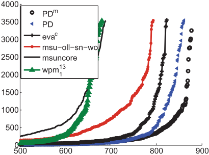
Tables 2-4 show that PRIMALDUALMAXSAT and PRIMALDUALMIN significantly improve over other solvers in the majority of benchmarks, solving more instances and using less time. For example, on 'pref. plan.' and 'One path' benchmarks, PRIMALDUALMIN is about three times faster than evac , msuoll and msunc. Our algorithms also solve significantly more instances in 'Multiple path' and 'msp' sets compared to other solvers. Note also that our use of minimization does not help in the MAXSAT category, but is useful in the two other categories. Table 1 gives a pairwise comparison between all pairs of the algorithms and Figure 1 shows a cactus plot over all industrial instances. Table 1 illustrates that PRIMALDUALMIN solves almost all problems also solved by other solvers, and other solvers do not offer any significant edge. For example, evac can only solve 7 instances not solved by PRIMALDUALMIN, while PRIMALDUALMIN solves 61 problems not solved by evac .
Conclusions
We developed a new iterative algorithm for MAXSAT that solves MAXSAT using a sequence of SAT and UNSAT formulas. We investigated theoretical properties of the algorithm and demonstrated its efficiency on a wide range of industrial
# l d
Figure 1: The cactus plot for all industrial instances from the 2014 Evaluation of MaxSAT Solvers competition.
benchmarks from the 2014 Evaluation of Max-SAT Solvers.
| PDm | PD | evac | msuoll | msunc | wpm13 1 | |||||||
|---|---|---|---|---|---|---|---|---|---|---|---|---|
| # | avg t | # | avg t | # | avg t | # | avg t | # | avg t | # | avg t | |
| haplotyping | 98 | 51.1 | 97 | 19.0 | 95 | 32.8 | 97 | 370.6 | 60 | 589.8 | 92 | 130.6 |
| hs-time. | 1 | 176.0 | 1 | 342.0 | 2 | 1202.0 | 1 | 123.0 | 1 | 1130.0 | 0 | 0.0 |
| packup | 97 | 16.5 | 95 | 35.6 | 89 | 45.1 | 69 | 170.4 | 28 | 208.5 | 90 | 26.3 |
| pref. plan. | 29 | 51.1 | 29 | 36.6 | 29 | 125.6 | 27 | 230.0 | 28 | 175.3 | 27 | 58.1 |
| timetabling | 12 | 618.8 | 13 | 554.7 | 11 | 285.1 | 10 | 616.7 | 8 | 272.5 | 8 | 687.5 |
| upgrad. | 100 | 1.2 | 100 | 0.9 | 100 | 44.1 | 100 | 128.4 | 100 | 128.2 | 100 | 6.2 |
| wcsp.dir | 14 | 1.6 | 14 | 1.2 | 14 | 5.9 | 14 | 95.4 | 11 | 35.2 | 14 | 124.4 |
| wcsp.log | 14 | 12.5 | 13 | 378.3 | 14 | 90.3 | 14 | 37.6 | 12 | 316.8 | 14 | 527.6 |
| Total | 365 | 43.9 | 362 | 52.1 | 354 | 62.3 | 332 | 225.6 | 248 | 267.9 | 345 | 90.4 |
@inproceedings{ijcai2015p41,
  title     = {Maximum Satisfiability Using Cores and Correction Sets},
  author    = {Bjørner, Nikolaj S. and Narodytska, Nina},
  booktitle = {Proceedings of the Twenty-Fourth International Joint Conference on
               Artificial Intelligence, {IJCAI-15}},
  publisher = {International Joint Conferences on Artificial Intelligence},
  editor    = {Qiang Yang and Michael Wooldridge},
  pages     = {246--251},
  year      = {2015},
  month     = {7},
  note      = {Main Track},
  url       = {https://ijcai.org/proceedings/2015/41},
}
TY - CPAPER TI - Maximum Satisfiability Using Cores and Correction Sets AU - Bjørner, Nikolaj S. AU - Narodytska, Nina T2 - Proceedings of the Twenty-Fourth International Joint Conference on Artificial Intelligence, IJCAI-15 PB - International Joint Conferences on Artificial Intelligence PY - 2015 SP - 246 EP - 251 UR - https://ijcai.org/proceedings/2015/41 ER -Copied
Machine-readable versions of this paper, for tools and AI agents:





